Original version: 31 October, 2023
Introduction
This vignette illustrates how to display AlphaMissense predictions on AlphaFold predicted protein structure.
Visualization makes use of CRAN packages bio3d and r3dmol. Install these (if necessary) with
pkgs <- c("bio3d", "r3dmol")
pkgs_to_install <- pkgs[!pkgs %in% rownames(installed.packages())]
if (length(pkgs_to_install))
    BiocManager::install(pkgs_to_install)
Start by loading the AlphaMissenseR library.
Visit the summary of available AlphaMissense datasets
am_available()
#> # A tibble: 7 × 6
#>   record   key                             size cached filename            link
#>   <chr>    <chr>                          <dbl> <lgl>  <chr>               <chr>
#> 1 10813168 gene_hg38                     253636 TRUE   AlphaMissense_gene… http…
#> 2 10813168 isoforms_hg38             1177361934 FALSE  AlphaMissense_isof… http…
#> 3 10813168 isoforms_aa_substitutions 2461351945 FALSE  AlphaMissense_isof… http…
#> 4 10813168 hg38                       642961469 TRUE   AlphaMissense_hg38… http…
#> 5 10813168 hg19                       622293310 FALSE  AlphaMissense_hg19… http…
#> 6 10813168 gene_hg19                     243943 FALSE  AlphaMissense_gene… http…
#> 7 10813168 aa_substitutions          1207278510 TRUE   AlphaMissense_aa_s… http…
This vignette uses the aa_substitutions and
hg38 data resources; make sure that these have been cached
locally.
am_data("aa_substitutions")
#> # Source:   table<aa_substitutions> [?? x 4]
#> # Database: DuckDB 1.4.2 [mtmorgan@Darwin 25.1.0:R 4.6.0//Users/mtmorgan/Library/Caches/org.R-project.R/R/BiocFileCache/785c21cda4e0_785c21cda4e0]
#>    uniprot_id protein_variant am_pathogenicity am_class
#>    <chr>      <chr>                      <dbl> <chr>
#>  1 A0A024R1R8 M1A                        0.467 ambiguous
#>  2 A0A024R1R8 M1C                        0.383 ambiguous
#>  3 A0A024R1R8 M1D                        0.827 pathogenic
#>  4 A0A024R1R8 M1E                        0.524 ambiguous
#>  5 A0A024R1R8 M1F                        0.275 benign
#>  6 A0A024R1R8 M1G                        0.548 ambiguous
#>  7 A0A024R1R8 M1H                        0.552 ambiguous
#>  8 A0A024R1R8 M1I                        0.321 benign
#>  9 A0A024R1R8 M1K                        0.288 benign
#> 10 A0A024R1R8 M1L                        0.175 benign
#> # ℹ more rows
am_data("hg38")
#> # Source:   table<hg38> [?? x 10]
#> # Database: DuckDB 1.4.2 [mtmorgan@Darwin 25.1.0:R 4.6.0//Users/mtmorgan/Library/Caches/org.R-project.R/R/BiocFileCache/785c21cda4e0_785c21cda4e0]
#>    CHROM   POS REF   ALT   genome uniprot_id transcript_id     protein_variant
#>    <chr> <dbl> <chr> <chr> <chr>  <chr>      <chr>             <chr>
#>  1 chr1  69094 G     T     hg38   Q8NH21     ENST00000335137.4 V2L
#>  2 chr1  69094 G     C     hg38   Q8NH21     ENST00000335137.4 V2L
#>  3 chr1  69094 G     A     hg38   Q8NH21     ENST00000335137.4 V2M
#>  4 chr1  69095 T     C     hg38   Q8NH21     ENST00000335137.4 V2A
#>  5 chr1  69095 T     A     hg38   Q8NH21     ENST00000335137.4 V2E
#>  6 chr1  69095 T     G     hg38   Q8NH21     ENST00000335137.4 V2G
#>  7 chr1  69097 A     G     hg38   Q8NH21     ENST00000335137.4 T3A
#>  8 chr1  69097 A     C     hg38   Q8NH21     ENST00000335137.4 T3P
#>  9 chr1  69097 A     T     hg38   Q8NH21     ENST00000335137.4 T3S
#> 10 chr1  69098 C     A     hg38   Q8NH21     ENST00000335137.4 T3N
#> # ℹ more rows
#> # ℹ 2 more variables: am_pathogenicity <dbl>, am_class <chr>
AlphaFold protein structure
AlphaMissense predictions on pathogenicity of amino acid changes can be combined with AlphaFold (or other) predictions of protein structure.
Fast path
Figure 3F of the AlphaMissense publication visualizes mean pathogenicity for UniProt id P35557. Filter amino acid data for that identifier
and visualization median pathogenicity with
af_prediction_view(P35557_aa)The image is interactive, including rotation and zoom. The following sections explore this visualization in more detail.
UniProt identifiers
Both AlphaMissense and AlphaFold use UniProt identifiers. Find all
AlphaMissense amino acid substitutions with UniProt identifiers starting
with P3555; the choice of this identifier is so that
results can be compared with Figure 3F of the AlphaMissense
publication.
uniprot_ids <-
    am_data("aa_substitutions") |>
    dplyr::filter(uniprot_id %like% "P3555%") |>
    dplyr::distinct(uniprot_id) |>
    pull(uniprot_id)
uniprot_ids
#> [1] "P35556" "P35555" "P35558" "P35557"
The AlphaMissenseR
package includes several functions that facilitate interaction with AlphaFold; these functions start
with af_*(). Use af_predictions() to discover
AlphaFold predictions (via the AlphaFold API) associated with UniProt
identifiers.
prediction <- af_predictions(uniprot_ids)
#> * [14:46:35][info] 1 of 4 uniprot accessions not found
#>   'P35555'
glimpse(prediction)
#> Rows: 2
#> Columns: 39
#> $ toolUsed                   <chr> "AlphaFold Monomer v2.0 pipeline", "AlphaFo…
#> $ providerId                 <chr> "GDM", "GDM"
#> $ entityType                 <chr> "protein", "protein"
#> $ isUniProt                  <lgl> TRUE, TRUE
#> $ modelEntityId              <chr> "AF-P35558-F1", "AF-P35557-F1"
#> $ modelCreatedDate           <chr> "2025-08-01T00:00:00Z", "2025-08-01T00:00:0…
#> $ sequenceVersionDate        <chr> "2006-03-07T00:00:00Z", "1994-06-01T00:00:0…
#> $ globalMetricValue          <dbl> 96.44, 93.69
#> $ fractionPlddtVeryLow       <dbl> 0.003, 0.002
#> $ fractionPlddtLow           <dbl> 0.011, 0.019
#> $ fractionPlddtConfident     <dbl> 0.048, 0.133
#> $ fractionPlddtVeryHigh      <dbl> 0.937, 0.845
#> $ latestVersion              <int> 6, 6
#> $ allVersions                <list> [1, 2, 3, 4, 5, 6], [1, 2, 3, 4, 5, 6]
#> $ sequence                   <chr> "MPPQLQNGLNLSAKVVQGSLDSLPQAVREFLENNAELCQPDH…
#> $ sequenceStart              <int> 1, 1
#> $ sequenceEnd                <int> 622, 465
#> $ sequenceChecksum           <chr> "78D309E0845CC181", "094D4A2F78096724"
#> $ isUniProtReviewed          <lgl> TRUE, TRUE
#> $ gene                       <chr> "PCK1", "GCK"
#> $ uniprotAccession           <chr> "P35558", "P35557"
#> $ uniprotId                  <chr> "PCKGC_HUMAN", "HXK4_HUMAN"
#> $ uniprotDescription         <chr> "Phosphoenolpyruvate carboxykinase, cytosol…
#> $ taxId                      <int> 9606, 9606
#> $ organismScientificName     <chr> "Homo sapiens", "Homo sapiens"
#> $ isUniProtReferenceProteome <lgl> TRUE, TRUE
#> $ bcifUrl                    <chr> "https://alphafold.ebi.ac.uk/files/AF-P3555…
#> $ cifUrl                     <chr> "https://alphafold.ebi.ac.uk/files/AF-P3555…
#> $ pdbUrl                     <chr> "https://alphafold.ebi.ac.uk/files/AF-P3555…
#> $ paeImageUrl                <chr> "https://alphafold.ebi.ac.uk/files/AF-P3555…
#> $ msaUrl                     <chr> "https://alphafold.ebi.ac.uk/files/msa/AF-P…
#> $ plddtDocUrl                <chr> "https://alphafold.ebi.ac.uk/files/AF-P3555…
#> $ paeDocUrl                  <chr> "https://alphafold.ebi.ac.uk/files/AF-P3555…
#> $ entryId                    <chr> "AF-P35558-F1", "AF-P35557-F1"
#> $ uniprotSequence            <chr> "MPPQLQNGLNLSAKVVQGSLDSLPQAVREFLENNAELCQPDH…
#> $ uniprotStart               <int> 1, 1
#> $ uniprotEnd                 <int> 622, 465
#> $ isReferenceProteome        <lgl> TRUE, TRUE
#> $ isReviewed                 <lgl> TRUE, TRUE
Note the message indicating that some UniProt identifiers
(accessions) are not found in the AlphaFold database. The query returns
a tibble containing columns with information on organism and UniProt
characteristics (including protein sequence) , as well as URLs for files
representing three-dimensional protein structure. We will use
pdbUrl.
Protein structure
Focus on a particular UniProt identifier and the PDB url.
Cache the PDB file using BiocFileCache, and read the PDB file using bio3d.
pdb_file <- BiocFileCache::bfcrpath(rnames = basename(pdb_url), fpath = pdb_url)
pdb <- bio3d::read.pdb(pdb_file)
pdb
#>
#>  Call:  bio3d::read.pdb(file = pdb_file)
#>
#>    Total Models#: 1
#>      Total Atoms#: 3642,  XYZs#: 10926  Chains#: 1  (values: A)
#>
#>      Protein Atoms#: 3642  (residues/Calpha atoms#: 465)
#>      Nucleic acid Atoms#: 0  (residues/phosphate atoms#: 0)
#>
#>      Non-protein/nucleic Atoms#: 0  (residues: 0)
#>      Non-protein/nucleic resid values: [ none ]
#>
#>    Protein sequence:
#>       MLDDRARMEAAKKEKVEQILAEFQLQEEDLKKVMRRMQKEMDRGLRLETHEEASVKMLPT
#>       YVRSTPEGSEVGDFLSLDLGGTNFRVMLVKVGEGEEGQWSVKTKHQMYSIPEDAMTGTAE
#>       MLFDYISECISDFLDKHQMKHKKLPLGFTFSFPVRHEDIDKGILLNWTKGFKASGAEGNN
#>       VVGLLRDAIKRRGDFEMDVVAMVNDTVATMISCYYEDHQCEVGMI...<cut>...MLGQ
#>
#> + attr: atom, xyz, seqres, calpha, call
Visualize the protein using r3dmol, using the ‘cartoon’ style.
r3dmol::r3dmol() |>
    ## use the PDB representation
    r3dmol::m_add_model(r3dmol::m_bio3d(pdb)) |>
    ## visualize as a 'cartoon' with alpha helices and beta sheets
    r3dmol::m_set_style(style = r3dmol::m_style_cartoon(arrow = TRUE)) |>
    ## fit molecule into display area
    r3dmol::m_zoom_to()
Average pathogenicity
Our goal is to visualize some measure of ‘average’ pathogenicity on
the three-dimensional protein structure provided by AlphaFold. Start
with a specific genome sequence (e.g., hg38). Filter to the
amino acids in our UniProt region of interest.
At each chromosome position, the AlphaMissense predictions contain several alternative alleles and hence protein variants. The (arithmetic) average pathogenicity (this is an extremely naive computation) at each amino acid position is
pathogenicity <- am_aa_pathogenicity(P35557)
pathogenicity
#> # A tibble: 464 × 9
#>    uniprot_id aa_pos aa_ref aa_pathogenicity_n aa_pathogenicity_mean
#>    <chr>       <int> <chr>               <int>                 <dbl>
#>  1 P35557          2 L                       5                0.0818
#>  2 P35557          3 D                       8                0.184
#>  3 P35557          4 D                       8                0.147
#>  4 P35557          5 R                       6                0.250
#>  5 P35557          6 A                       6                0.138
#>  6 P35557          7 R                       7                0.257
#>  7 P35557          8 M                       9                0.142
#>  8 P35557          9 E                       7                0.212
#>  9 P35557         10 A                       6                0.142
#> 10 P35557         11 A                       6                0.142
#> # ℹ 454 more rows
#> # ℹ 4 more variables: aa_pathogenicity_median <dbl>,
#> #   aa_pathogenicity_min <dbl>, aa_pathogenicity_max <dbl>,
#> #   aa_pathogenicity_mode <fct>
Coloring amino acids by position
Individual amino acids can be colored using the
colorfunc= argument to
r3dmol::m_style_cartoon(). This is a Javascript function
that takes each atom position and returns the corresponding color. The
approach taken in AlphaMissenseR is
to use a template, ultimately replacing ... with a vector
of residue colors.
cat(
    AlphaMissenseR:::js_template("colorfunc", colors = "..."),
    "\n"
)
#> function(atom) {
#>     const residue_colors = [ ... ];
#>     return residue_colors[atom.resi];
#> }
The function af_colorfunc_by_position() provides a
mechanism for translating a vector of scores between zero and one into a
vector of colors. This is illustrated for a 12-amino acid sequence where
the first and last residues are uncolored.
df <- tibble(
    pos = 1 + 1:10, # no color information for position 1
    value = 10:1 / 10
)
colorfunc <- af_colorfunc_by_position(
    df,
    "pos", "value",
    pos_max = 12    # no color information for position 12
)
cat(colorfunc, "\n")
#> function(atom) {
#>     const residue_colors = [ 'gray', '#8E063B', '#AB5468', '#C18692', '#D2B0B6', '#DDD0D2', '#D2D3DC', '#B3B7CF', '#8C94BF', '#5D6CAE', '#023FA5', 'gray' ];
#>     return residue_colors[atom.resi];
#> }
The following color function is similar to that used in
af_prediction_view(), but uses the mean rather than median
pathogenicity and scales the palette between the minimum and maximum
values of the mean pathogenicity vector, rather than between 0 and
1.
colorfunc <-
    pathogenicity |>
    af_colorfunc_by_position(
        "aa_pos", "aa_pathogenicity_mean",
        length(pdb$seqres)
    )
Add this as the colorfunc= argument to
m_style_cartoon() for visualization.
r3dmol::r3dmol() |>
    ## use the PDB representation
    r3dmol::m_add_model(r3dmol::m_bio3d(pdb)) |>
    ## visualize as a 'cartoon' with alpha helices and beta sheets
    r3dmol::m_set_style(
        style = r3dmol::m_style_cartoon(
            arrow = TRUE,
            ## color residue according to colorfunc
            colorfunc = colorfunc
        )
    ) |>
    ## fit molecule into display area
    r3dmol::m_zoom_to()
Visualizing genomic tracks
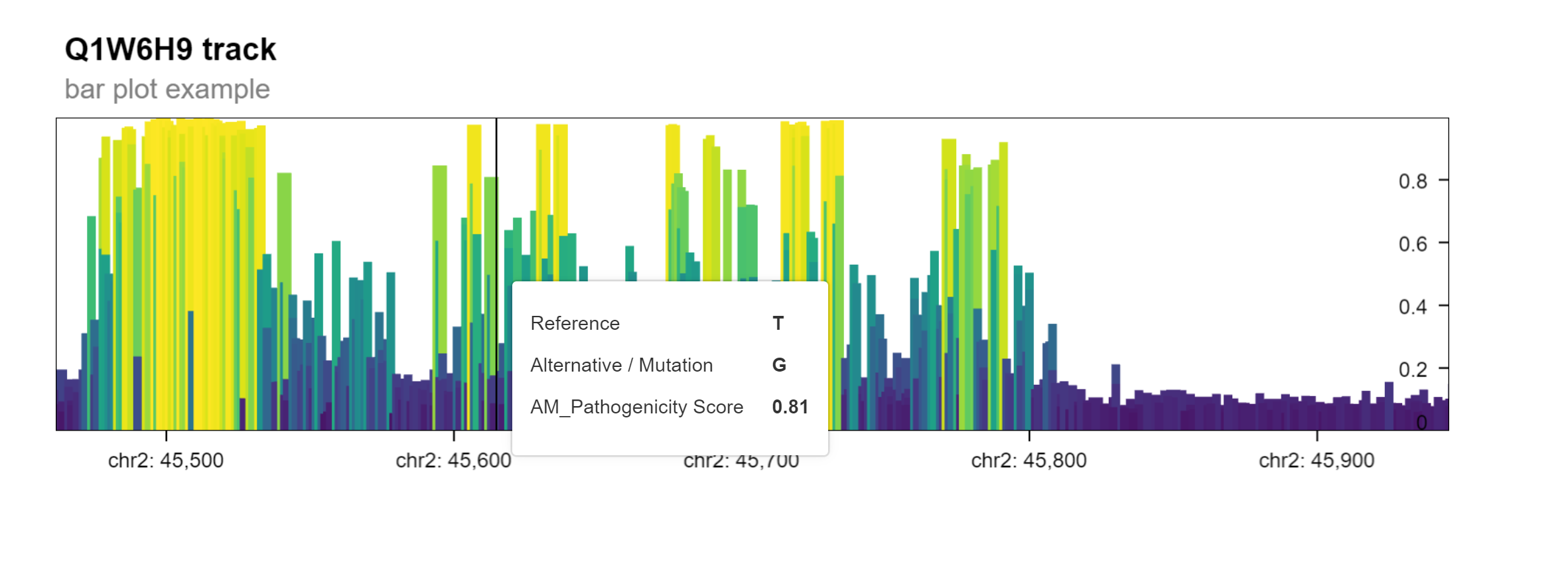
The variant effect prediction data can also be visualized in a genome browser view. This allows the user to explore the predicted pathogenicity of single nucleotide missense mutations in a gene of interest. This multi-scale visualization is based on Gosling, a grammar-based toolkit for scalable and interactive genomics data visualization.
For demonstration, we create a GPos object for a protein
of interest.
The function plot_granges invokes functionality from the
shiny.gosling
package to produce an interactive genome track plot in which the
pathogenicity score for each point mutation in a linear genomic
track.
The resulting plot is a Shiny app that can be displayed when running the following command in an interactive R session.
gosling_plot(
    gpos, plot_type = "bar",
    title = "Q1W6H9 track",
    subtitle = "bar plot example"
)
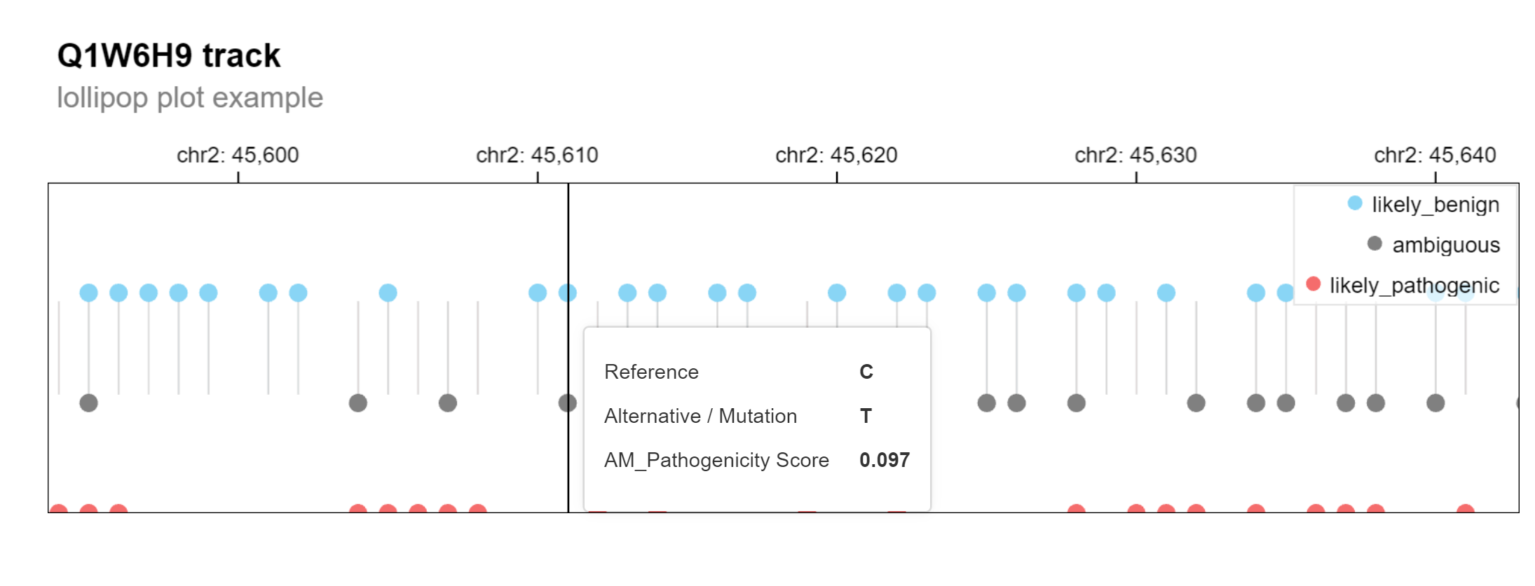
Alternatively, a multiscale-lollipop plot can be generated with the
same function by changing the plot_type argument to
highlight the predicted class outcomes for each mutation (ambigious,
benign, pathogenic).
gosling_plot(
    gpos, plot_type = "lollipop",
    title = "Q1W6H9 track",
    subtitle = "lollipop plot example"
)
Finally
Remember to disconnect and shutdown all managed DuckDB connections.
db_disconnect_all()
#> * [14:46:37][info] disconnecting all registered connections
Database connections that are not closed correctly trigger warning messages.
Session information
sessionInfo()
#> R Under development (unstable) (2025-08-09 r88545)
#> Platform: aarch64-apple-darwin24.6.0
#> Running under: macOS Tahoe 26.1
#>
#> Matrix products: default
#> BLAS:   /Users/mtmorgan/bin/R-devel/lib/libRblas.dylib
#> LAPACK: /Users/mtmorgan/bin/R-devel/lib/libRlapack.dylib;  LAPACK version 3.12.1
#>
#> locale:
#> [1] en_CA.UTF-8/en_CA.UTF-8/en_CA.UTF-8/C/en_CA.UTF-8/en_CA.UTF-8
#>
#> time zone: America/Toronto
#> tzcode source: internal
#>
#> attached base packages:
#> [1] stats     graphics  grDevices utils     datasets  methods   base
#>
#> other attached packages:
#> [1] AlphaMissenseR_1.7.1 dplyr_1.1.4
#>
#> loaded via a namespace (and not attached):
#>  [1] gtable_0.3.6         xfun_0.54            bslib_0.9.0
#>  [4] ggplot2_4.0.1        httr2_1.2.1          htmlwidgets_1.6.4
#>  [7] vctrs_0.6.5          rjsoncons_1.3.2      tools_4.6.0
#> [10] generics_0.1.4       stats4_4.6.0         curl_7.0.0
#> [13] parallel_4.6.0       tibble_3.3.0         RSQLite_2.4.4
#> [16] blob_1.2.4           shiny.gosling_1.5.0  pkgconfig_2.0.3
#> [19] BiocBaseUtils_1.12.0 dbplyr_2.5.1         RColorBrewer_1.1-3
#> [22] S4Vectors_0.48.0     S7_0.2.1             desc_1.4.3
#> [25] RcppSpdlog_0.0.23    lifecycle_1.0.4      compiler_4.6.0
#> [28] farver_2.1.2         textshaping_1.0.4    Seqinfo_1.0.0
#> [31] GenomeInfoDb_1.46.0  httpuv_1.6.16        htmltools_0.5.8.1
#> [34] sass_0.4.10          yaml_2.3.10          later_1.4.4
#> [37] pillar_1.11.1        pkgdown_2.2.0        jquerylib_0.1.4
#> [40] whisker_0.4.1        tidyr_1.3.1          cachem_1.1.0
#> [43] mime_0.13            tidyselect_1.2.1     r3dmol_0.1.2
#> [46] digest_0.6.39        duckdb_1.4.2         purrr_1.2.0
#> [49] fastmap_1.2.0        grid_4.6.0           colorspace_2.1-2
#> [52] cli_3.6.5            magrittr_2.0.4       dichromat_2.0-0.1
#> [55] spdl_0.0.5           utf8_1.2.6           withr_3.0.2
#> [58] UCSC.utils_1.6.0     promises_1.5.0       filelock_1.0.3
#> [61] scales_1.4.0         rappdirs_0.3.3       bit64_4.6.0-1
#> [64] XVector_0.50.0       rmarkdown_2.30       httr_1.4.7
#> [67] otel_0.2.0           bit_4.6.0            ragg_1.5.0
#> [70] shiny_1.11.1         memoise_2.0.1        evaluate_1.0.5
#> [73] knitr_1.50           IRanges_2.44.0       GenomicRanges_1.62.0
#> [76] bio3d_2.4-5          BiocFileCache_3.0.0  rlang_1.1.6
#> [79] Rcpp_1.1.0           xtable_1.8-4         glue_1.8.0
#> [82] DBI_1.2.3            BiocGenerics_0.56.0  jsonlite_2.0.0
#> [85] R6_2.6.1             systemfonts_1.3.1    fs_1.6.6