Introduction to R

R is an interactive programming language emphasizing statistical analysis and visualization. It is very useful for both light-weight data manipulation, and for advanced statistical analysis and visualization. R is available as Free Software under the GNU General Public License. It is highly extensible through user-contributed ‘packages’, of which there are more than 20,000 available through CRAN (Comprehensive R Archive Network) and more than 2,000 through Bioconductor (for high-throughput genomic data).

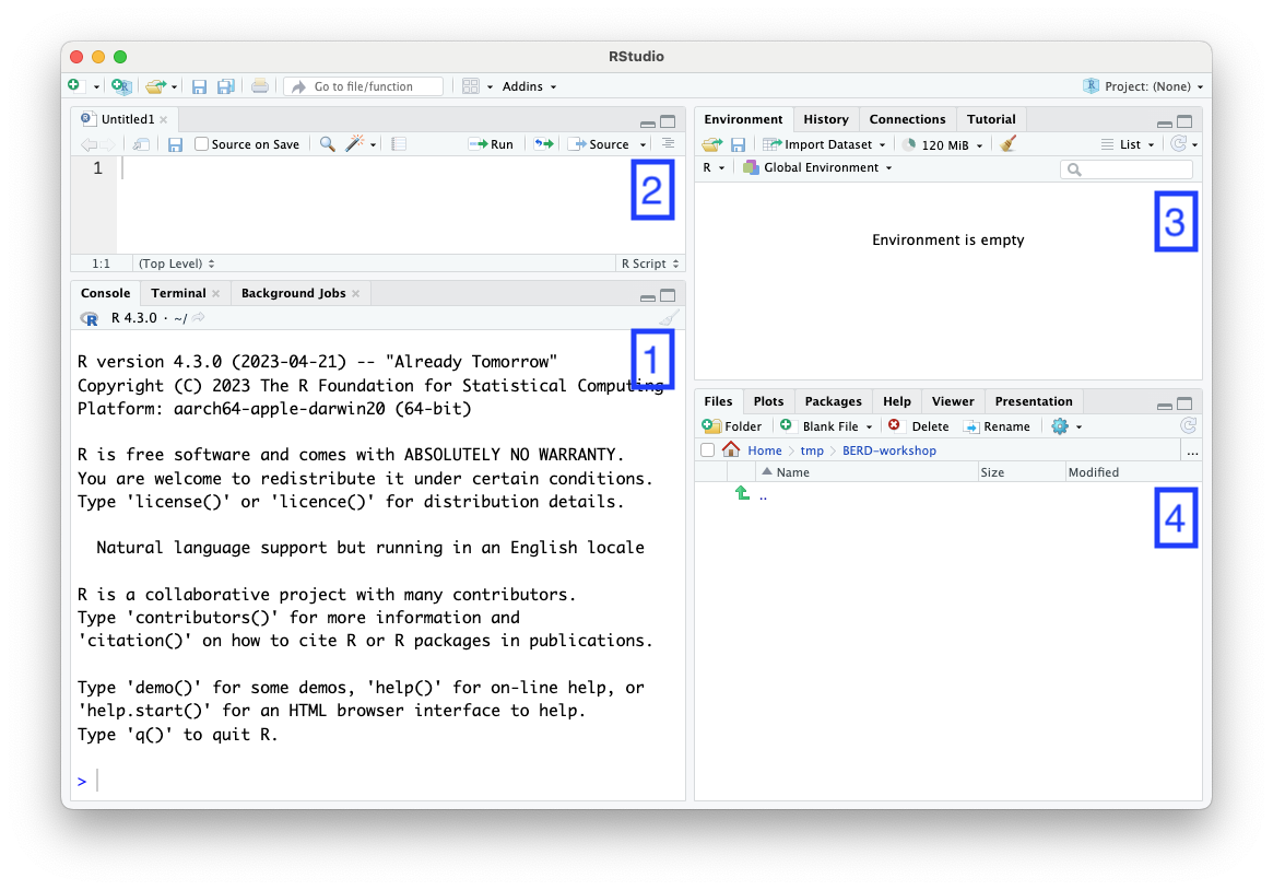
RStudio

1. Console

   

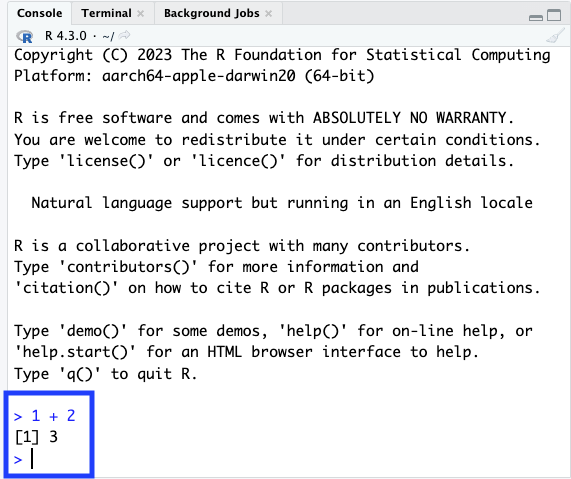
   • enter R code ‘interactively’ at the prompt >. Press ‘return’ to evaluate the code you have entered.

2. Scripts & ‘markdown’

   

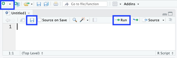
   • Enter R code here to save for later use.
   • Use the ‘+’ icon or RStudio ‘File’ menu item to create new script files. Use the ‘floppy disk’ icon to save the script file after changes.
   • Use the ‘Run’ icon to run commands in the script in the console.

3. Environment, history, …

   • Contains information about variables and commands created during an R session.

4. Files, plots, packages, help, …

   • Access to your computer file system, e.g., to open R scripts that you had previously saved.
   • Plot visualization, help pages, etc.

R

1 + 2
#> [1] 3

sqrt(2)
#> [1] 1.414214

Vectors and variables

R usually works on vectors of values

c(1, 2, 3)
#> [1] 1 2 3

It usually makes sense to assign a vector of values to a variable, to make it easy to repeatedly reference the same set of values

x <- c(1, 2, 3)
x
#> [1] 1 2 3

Types of vectors

• logical – c(TRUE, FALSE)
• integer – c(1, 2, 3)
• numeric – c(1.41, 2.30, 3.14159)
• character – c("May", "June", "July")
• complex

Statistical concepts

• ‘Missing’ values
  • use NA in any vector, e.g., c(1, 2, NA, 3)
• factor with levels

  • Often, in an experimental design, there are defined number of groups, e.g., ‘treatment’ and ‘control’

  • Use a factor to represent these values

    levels <- c("treatment", "control") # possible values
    ## observed values -- four samples
    values <- c("treatment", "treatment", "control", "control")
    factor(values, levels = levels)
    #> [1] treatment treatment control   control  
    #> Levels: treatment control

Operations, e.g., numeric

• two vectors – element-wise

  x <- c(1, 2, 3)
  y <- c(4, 5, 6)
  x + y
  #> [1] 5 7 9

• vector and scalar – scalar is ‘recycled’ to the same length as vector, and then element-wise operations are preformed

  x * 2
  #> [1] 2 4 6

Common operations

• logical – & (‘and’), | (‘or’), ! (not), == (element-wise equivalence)

  c(TRUE, TRUE, FALSE, FALSE) & c(TRUE, FALSE, TRUE, FALSE)
  #> [1]  TRUE FALSE FALSE FALSE
  c(TRUE, TRUE, FALSE, FALSE) | c(TRUE, FALSE, TRUE, FALSE)
  #> [1]  TRUE  TRUE  TRUE FALSE
  !c(TRUE, TRUE, FALSE, FALSE)
  #> [1] FALSE FALSE  TRUE  TRUE
  c(TRUE, TRUE, FALSE, FALSE) == c(TRUE, FALSE, TRUE, FALSE)
  #> [1]  TRUE FALSE FALSE  TRUE
  ## Fun!
  c(TRUE, FALSE, NA) & c(NA, NA, NA)
  #> [1]    NA FALSE    NA
  c(TRUE, FALSE, NA) | c(NA, NA, NA)
  #> [1] TRUE   NA   NA

• integer / numeric – +, -, *. Comparison ==, >, >=, <, <=. Many functions like log(), sqrt(), …

• character – paste() (paste two string togther), nchar(), substring()

  month <- c("April", "May", "June", "July")
  year <- c("2020", "2021", "2022", "2023")
  paste(year, month)
  #> [1] "2020 April" "2021 May"   "2022 June"  "2023 July"

Subsetting

x <- c(1, 2, 3, 4)
x[c(1, 3)]
#> [1] 1 3
x[x >= 3]
#> [1] 3 4

data.frame

Organizing vectors into columns

df <- data.frame(
    Month = month, Year = year,
    Temperature = c(20, 22, 24, 25)
)
df
#>   Month Year Temperature
#> 1 April 2020          20
#> 2   May 2021          22
#> 3  June 2022          24
#> 4  July 2023          25

Subsetting

• columns

  df[, c("Month", "Temperature")]
  #>   Month Temperature
  #> 1 April          20
  #> 2   May          22
  #> 3  June          24
  #> 4  July          25

• rows

  df[c(1, 3), ]
  #>   Month Year Temperature
  #> 1 April 2020          20
  #> 3  June 2022          24

Column access

• $; can be useful to subset

  df$Temperature
  #> [1] 20 22 24 25
  df[df$Temperature > 22,]
  #>   Month Year Temperature
  #> 3  June 2022          24
  #> 4  July 2023          25

• [[; useful when a variable defines the column of interest

  column_of_interest <- "Temperature"
  df[[ column_of_interest ]]
  #> [1] 20 22 24 25

Functions

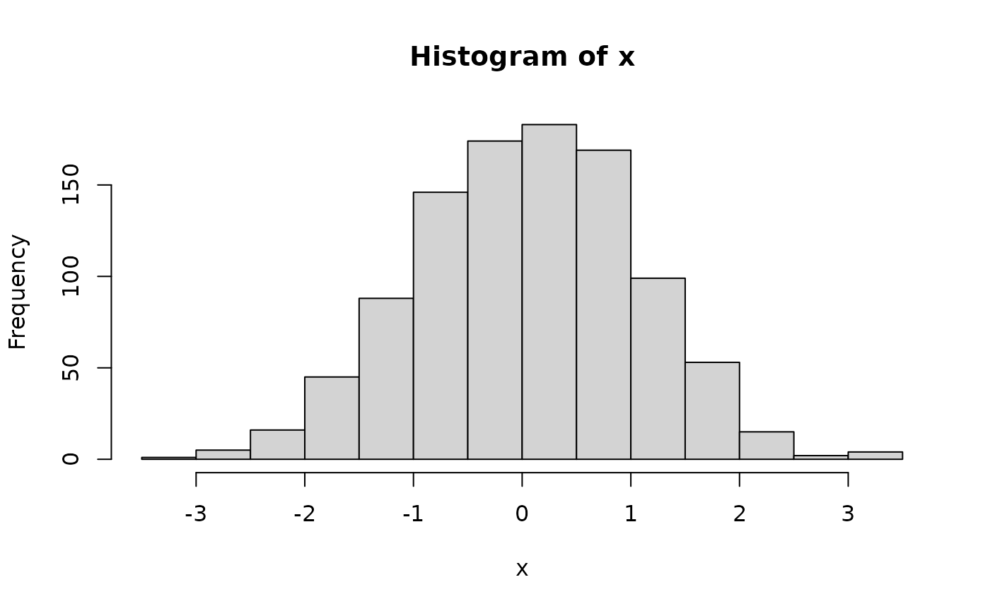
x <- rnorm(100)
x
#>   [1]  0.20026483 -2.08047904 -0.45978334 -1.08842623  0.19215992  0.50257165
#>   [7] -0.62152096 -0.93928405  1.86501268  0.44614855 -0.08610675  0.55179653
#>  [13]  1.03282317 -0.64070706 -2.14296764  0.66958672 -0.26214000  1.57563947
#>  [19] -1.25630130  0.58029938 -0.66471898 -0.56243673 -0.49918936  0.01925961
#>  [25] -0.31582955 -0.92930561  0.29581233  0.58671999 -1.51076917 -0.94404124
#>  [31]  0.05820170  0.32634754  0.57226754 -1.36155627 -0.14544117  0.82568822
#>  [37] -0.38770719  0.87980959  1.63456139 -0.12202832 -0.19302331 -0.05396342
#>  [43] -1.05099061 -0.70724939  0.13189819 -1.06644246 -1.35711429 -0.23227926
#>  [49] -2.13089098  0.15972191  2.06951808 -0.90941254 -0.99683200  1.91832622
#>  [55] -2.00506397 -0.50844600  1.42340708  2.12161178  2.28316982 -1.89608228
#>  [61] -0.74622632 -0.15585202  0.50912319 -0.44967120 -1.38776833 -0.64652418
#>  [67] -0.19881017  0.88777352 -0.10288515  1.45557676  0.99781736 -0.15770456
#>  [73] -0.83088916 -0.99295025 -0.91327025  0.67009803  0.54755717 -2.02572927
#>  [79]  0.94921115  0.42001286 -0.84146370 -0.51355204  0.35458312  0.42797770
#>  [85]  0.72909443 -0.80888531  0.14153530  0.76902868 -0.44591538 -0.86688965
#>  [91]  0.14450450 -0.87450025 -0.32575753  0.24620252 -0.13111425 -0.27878560
#>  [97]  1.45377740 -0.14846619  0.07746273  0.34118695

Look up the help page for rnorm – ?rnorm

Plot a histogram using hist()

x <- rnorm(1000)
hist(x)

Generate two equal-length vectors and visualize as a scatter plot

y <- x + rnorm(1000) # element-wise addition; each element of 'y' is
                     # the sum of two random variables
plot(x, y)           # one way to plot

plot(y ~ x)          # another way to plot -- 'y as a function of x'

Place x and y into a data.frame, and use to plot

df <- data.frame(X = x, Y = y)
plot(Y ~ X, df)

Subset to just the positive quadrant

plot(Y ~ X, df[df$X > 0 & df$Y > 0,])

A built-in data frame – mtcars

mtcars
#>                      mpg cyl  disp  hp drat    wt  qsec vs am gear carb
#> Mazda RX4           21.0   6 160.0 110 3.90 2.620 16.46  0  1    4    4
#> Mazda RX4 Wag       21.0   6 160.0 110 3.90 2.875 17.02  0  1    4    4
#> Datsun 710          22.8   4 108.0  93 3.85 2.320 18.61  1  1    4    1
#> Hornet 4 Drive      21.4   6 258.0 110 3.08 3.215 19.44  1  0    3    1
#> Hornet Sportabout   18.7   8 360.0 175 3.15 3.440 17.02  0  0    3    2
#> Valiant             18.1   6 225.0 105 2.76 3.460 20.22  1  0    3    1
#> Duster 360          14.3   8 360.0 245 3.21 3.570 15.84  0  0    3    4
#> Merc 240D           24.4   4 146.7  62 3.69 3.190 20.00  1  0    4    2
#> Merc 230            22.8   4 140.8  95 3.92 3.150 22.90  1  0    4    2
#> Merc 280            19.2   6 167.6 123 3.92 3.440 18.30  1  0    4    4
#> Merc 280C           17.8   6 167.6 123 3.92 3.440 18.90  1  0    4    4
#> Merc 450SE          16.4   8 275.8 180 3.07 4.070 17.40  0  0    3    3
#> Merc 450SL          17.3   8 275.8 180 3.07 3.730 17.60  0  0    3    3
#> Merc 450SLC         15.2   8 275.8 180 3.07 3.780 18.00  0  0    3    3
#> Cadillac Fleetwood  10.4   8 472.0 205 2.93 5.250 17.98  0  0    3    4
#> Lincoln Continental 10.4   8 460.0 215 3.00 5.424 17.82  0  0    3    4
#> Chrysler Imperial   14.7   8 440.0 230 3.23 5.345 17.42  0  0    3    4
#> Fiat 128            32.4   4  78.7  66 4.08 2.200 19.47  1  1    4    1
#> Honda Civic         30.4   4  75.7  52 4.93 1.615 18.52  1  1    4    2
#> Toyota Corolla      33.9   4  71.1  65 4.22 1.835 19.90  1  1    4    1
#> Toyota Corona       21.5   4 120.1  97 3.70 2.465 20.01  1  0    3    1
#> Dodge Challenger    15.5   8 318.0 150 2.76 3.520 16.87  0  0    3    2
#> AMC Javelin         15.2   8 304.0 150 3.15 3.435 17.30  0  0    3    2
#> Camaro Z28          13.3   8 350.0 245 3.73 3.840 15.41  0  0    3    4
#> Pontiac Firebird    19.2   8 400.0 175 3.08 3.845 17.05  0  0    3    2
#> Fiat X1-9           27.3   4  79.0  66 4.08 1.935 18.90  1  1    4    1
#> Porsche 914-2       26.0   4 120.3  91 4.43 2.140 16.70  0  1    5    2
#> Lotus Europa        30.4   4  95.1 113 3.77 1.513 16.90  1  1    5    2
#> Ford Pantera L      15.8   8 351.0 264 4.22 3.170 14.50  0  1    5    4
#> Ferrari Dino        19.7   6 145.0 175 3.62 2.770 15.50  0  1    5    6
#> Maserati Bora       15.0   8 301.0 335 3.54 3.570 14.60  0  1    5    8
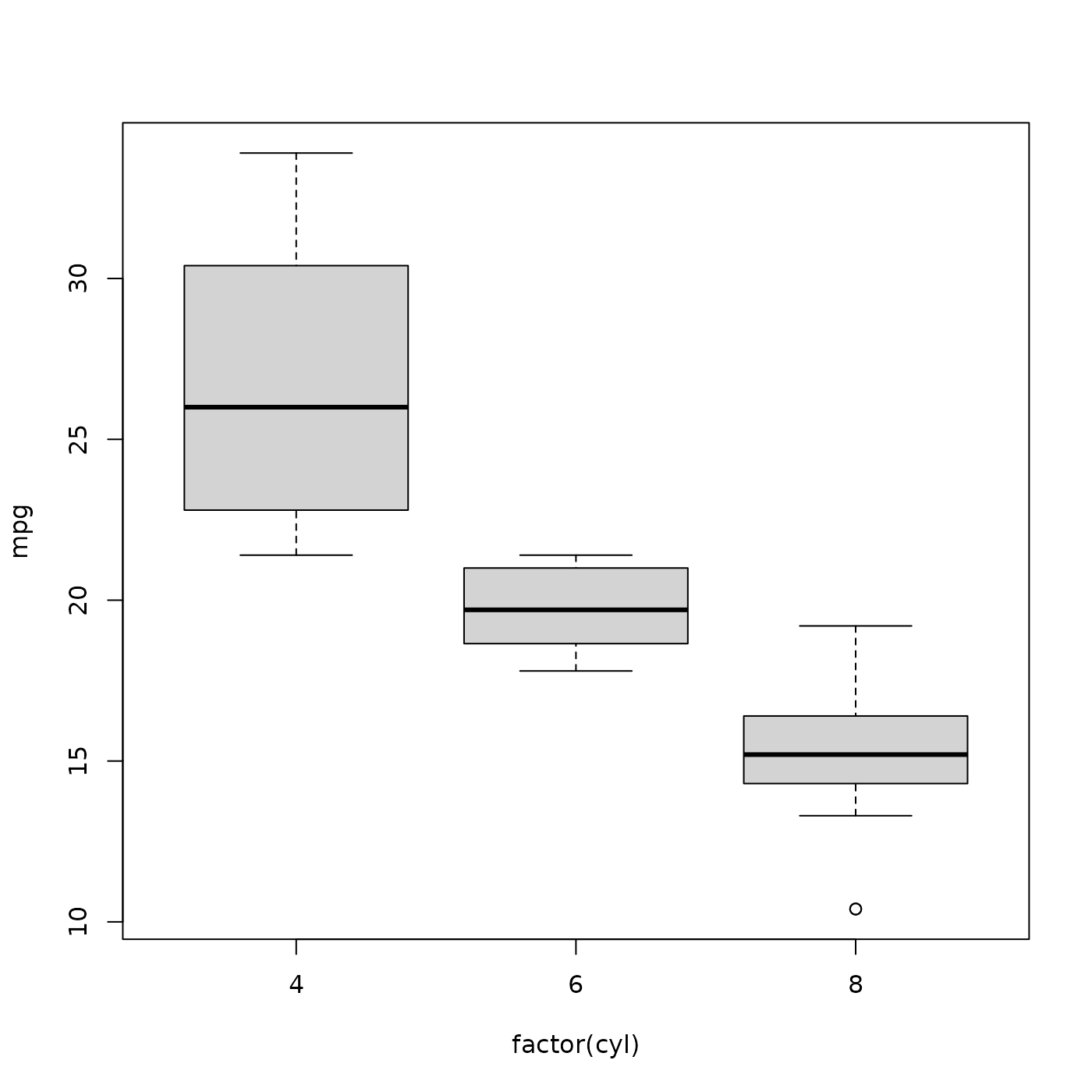
#> Volvo 142E          21.4   4 121.0 109 4.11 2.780 18.60  1  1    4    2

Plot miles per gallon mpg as a function of number of cylinders, cyl

plot(mpg ~ cyl, mtcars) # scatter plot

Note though that cyl should probably be a factor – a finite number of possible values.

mtcars$cyl
#>  [1] 6 6 4 6 8 6 8 4 4 6 6 8 8 8 8 8 8 4 4 4 4 8 8 8 8 4 4 4 8 6 8 4
factor(mtcars$cyl) # 'levels' have a sensible default
#>  [1] 6 6 4 6 8 6 8 4 4 6 6 8 8 8 8 8 8 4 4 4 4 8 8 8 8 4 4 4 8 6 8 4
#> Levels: 4 6 8

Treat cyl as a factor when plotting

plot(mpg ~ factor(cyl), mtcars)

Packages

Examples:

• dplyr: data manipulation based on ‘tidy’ principles.
• ggplot2: plotting using the ‘grammar of graphics’

Installation

• Packages only need to be installed once

  ## also possible to use RStudio 'Packages' panel...
  install.packages("dplyr", repos = "https://CRAN.R-project.org")

Use

• Attach packages in each R session where you would like to use it

  library(dplyr)

tibble versus data.frame

• only some values displayed – really useful even for this small data set

• column data types indicated

  tbl <- tibble(mtcars)
  tbl
  #> # A tibble: 32 × 11
  #>      mpg   cyl  disp    hp  drat    wt  qsec    vs    am  gear  carb
  #>    <dbl> <dbl> <dbl> <dbl> <dbl> <dbl> <dbl> <dbl> <dbl> <dbl> <dbl>
  #>  1  21       6  160    110  3.9   2.62  16.5     0     1     4     4
  #>  2  21       6  160    110  3.9   2.88  17.0     0     1     4     4
  #>  3  22.8     4  108     93  3.85  2.32  18.6     1     1     4     1
  #>  4  21.4     6  258    110  3.08  3.22  19.4     1     0     3     1
  #>  5  18.7     8  360    175  3.15  3.44  17.0     0     0     3     2
  #>  6  18.1     6  225    105  2.76  3.46  20.2     1     0     3     1
  #>  7  14.3     8  360    245  3.21  3.57  15.8     0     0     3     4
  #>  8  24.4     4  147.    62  3.69  3.19  20       1     0     4     2
  #>  9  22.8     4  141.    95  3.92  3.15  22.9     1     0     4     2
  #> 10  19.2     6  168.   123  3.92  3.44  18.3     1     0     4     4
  #> # ℹ 22 more rows

Pipes

• |> takes the value on the ‘left-hand side’ and uses it as the first argument in the function on the ‘right-hand side’

  tbl <-
      mtcars |>
      tibble()

• this can be a very useful paradigm – ‘take the mtcars data set, and apply the tibble function to it’ – and allows a series of related operations to be chained together

Help!!!

RStudio

R

• For help on individual commands, use ? at the command line, e.g., ?data.frame

• For package help, try

  vignette(package = "dplyr")
  #> Vignettes in package 'dplyr':
  #> 
  #> colwise                 Column-wise operations (source, html)
  #> base                    dplyr <-> base R (source, html)
  #> grouping                Grouped data (source, html)
  #> dplyr                   Introduction to dplyr (source, html)
  #> programming             Programming with dplyr (source, html)
  #> rowwise                 Row-wise operations (source, html)
  #> two-table               Two-table verbs (source, html)
  #> in-packages             Using dplyr in packages (source, html)
  #> window-functions        Window functions (source, html)
  #> 
  vignette(package = "dplyr", "dplyr")

Other sources of help

• Google

• StackOverflow

• ChatGPT & other AI

  • can be amazingly helpful, especially if asked to perform specific tasks
  • also useful to ‘explain this code’ or ‘add comments to this code’
  • what out for halucinations!

Session information

sessionInfo()
#> R version 4.3.3 (2024-02-29)
#> Platform: x86_64-pc-linux-gnu (64-bit)
#> Running under: Ubuntu 22.04.4 LTS
#> 
#> Matrix products: default
#> BLAS:   /usr/lib/x86_64-linux-gnu/openblas-pthread/libblas.so.3 
#> LAPACK: /usr/lib/x86_64-linux-gnu/openblas-pthread/libopenblasp-r0.3.20.so;  LAPACK version 3.10.0
#> 
#> locale:
#>  [1] LC_CTYPE=C.UTF-8       LC_NUMERIC=C           LC_TIME=C.UTF-8       
#>  [4] LC_COLLATE=C.UTF-8     LC_MONETARY=C.UTF-8    LC_MESSAGES=C.UTF-8   
#>  [7] LC_PAPER=C.UTF-8       LC_NAME=C              LC_ADDRESS=C          
#> [10] LC_TELEPHONE=C         LC_MEASUREMENT=C.UTF-8 LC_IDENTIFICATION=C   
#> 
#> time zone: UTC
#> tzcode source: system (glibc)
#> 
#> attached base packages:
#> [1] stats     graphics  grDevices utils     datasets  methods   base     
#> 
#> other attached packages:
#> [1] dplyr_1.1.4
#> 
#> loaded via a namespace (and not attached):
#>  [1] vctrs_0.6.5       cli_3.6.2         knitr_1.45        rlang_1.1.3      
#>  [5] xfun_0.43         highr_0.10        purrr_1.0.2       generics_0.1.3   
#>  [9] textshaping_0.3.7 jsonlite_1.8.8    glue_1.7.0        htmltools_0.5.8  
#> [13] ragg_1.3.0        sass_0.4.9        fansi_1.0.6       rmarkdown_2.26   
#> [17] tibble_3.2.1      evaluate_0.23     jquerylib_0.1.4   fastmap_1.1.1    
#> [21] yaml_2.3.8        lifecycle_1.0.4   memoise_2.0.1     compiler_4.3.3   
#> [25] fs_1.6.3          pkgconfig_2.0.3   systemfonts_1.0.6 digest_0.6.35    
#> [29] R6_2.5.1          tidyselect_1.2.1  utf8_1.2.4        pillar_1.9.0     
#> [33] magrittr_2.0.3    bslib_0.6.2       tools_4.3.3       pkgdown_2.0.7    
#> [37] cachem_1.0.8      desc_1.4.3