Example data: BRFSS
We use data from the US Center for Disease Control’s Behavioral Risk Factor Surveillance System (BRFSS) annual survey. Check out the web page for a little more information. We are using a small subset of this data, including a random sample of 20000 observations from each of 1990 and 2010.
Data input
From Excel to CSV
Getting a dataset into R is a necessary and sometimes tedious process. Often data starts as an Excel spreadsheet…
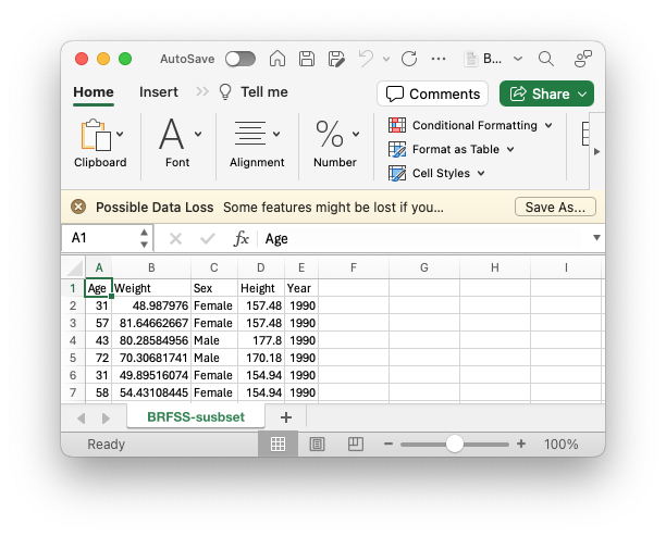
Note that this is a straight-forward sheet – the first row provides a column name. Each subsequent row corresponds to a single observation. There are no mouse-over ‘comments’ or secondary tables or… This simple structure is a good starting point for moving data to R.
Our first step is to export the data from Excel to a ‘CSV’ file. We do this because (a) CSV files are easily read into R and (b) many other data sources can be transformed to CSV format. Chose the ‘File’ menu and then ‘Save’. On macOS I then chose to save the data as CSV with a dialog box that looked like…
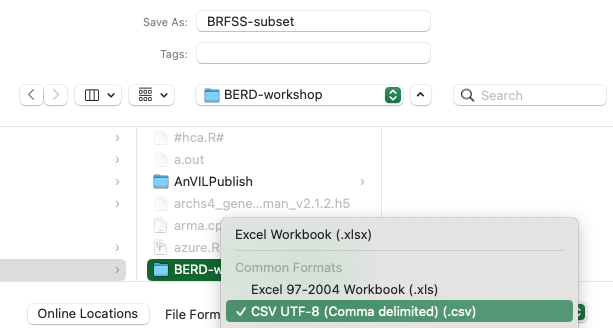
This procedure would create a file ‘BRFSS-subset.csv’ on our computer.
We can’t start with an Excel file, so instead download the data we
will work with using the following command. You might need to make sure
that the folder ‘BRFSS-workshop’ exists at the file system location
returned by getwd().
getwd()
url <- "https://raw.githubusercontent.com/mtmorgan/BERD/main/inst/extdata/BRFSS-subset.csv"
destination <- file.path("BRFSS-workshop", basename(url))
if (!file.exists(destination)) {
    dir.create("data")
    download.file(url, destination)
}
CSV to R
Read the data into R as a tibble using the readr package.
brfss <- readr::read_csv(destination)
#> Rows: 20000 Columns: 5
#> ── Column specification ────────────────────────────────────────────────────────
#> Delimiter: ","
#> chr (1): Sex
#> dbl (4): Age, Weight, Height, Year
#>
#> ℹ Use `spec()` to retrieve the full column specification for this data.
#> ℹ Specify the column types or set `show_col_types = FALSE` to quiet this message.
brfss
#> # A tibble: 20,000 × 5
#>      Age Weight Sex    Height  Year
#>    <dbl>  <dbl> <chr>   <dbl> <dbl>
#>  1    31   49.0 Female   157.  1990
#>  2    57   81.6 Female   157.  1990
#>  3    43   80.3 Male     178.  1990
#>  4    72   70.3 Male     170.  1990
#>  5    31   49.9 Female   155.  1990
#>  6    58   54.4 Female   155.  1990
#>  7    45   69.9 Male     173.  1990
#>  8    37   68.0 Male     180.  1990
#>  9    33   65.8 Female   170.  1990
#> 10    75   70.8 Female   152.  1990
#> # ℹ 19,990 more rows
Explore the data using dplyr
Attach dplyr to our current R session.
Useful functions for data exploration
-
count()– count occurence of values in one or more columns -
summarize()– more flexible summary of columns -
group_by()– summarize or perform other operations by group
Functions for data manipulation
-
mutate()– update or add columns -
filter()– remove rows based on column values -
select()– remove, rearrange, or re-name columns
count()
Count of observed values for one…
brfss |>
    count(Year)
#> # A tibble: 2 × 2
#>    Year     n
#>   <dbl> <int>
#> 1  1990 10000
#> 2  2010 10000
brfss |>
    count(Sex)
#> # A tibble: 2 × 2
#>   Sex        n
#>   <chr>  <int>
#> 1 Female 12039
#> 2 Male    7961
…or several columns
brfss |>
    count(Year, Sex)
#> # A tibble: 4 × 3
#>    Year Sex        n
#>   <dbl> <chr>  <int>
#> 1  1990 Female  5718
#> 2  1990 Male    4282
#> 3  2010 Female  6321
#> 4  2010 Male    3679
summarize()
More flexible summary, e.g., number of observations n()
or mean values of columns, removing NA,
mean(, na.rm = TRUE).
group_by()
Often data sets contain groups that can be summarized separately, e.g., calculating mean values by Year and Sex.
brfss |>
    group_by(Year, Sex) |>
    summarize(
        n = n(),
        ave_age = mean(Age, na.rm = TRUE),
        ave_wt = mean(Weight, na.rm = TRUE),
        ave_ht = mean(Height, na.rm = TRUE)
    )
#> `summarise()` has grouped output by 'Year'. You can override using the
#> `.groups` argument.
#> # A tibble: 4 × 6
#> # Groups:   Year [2]
#>    Year Sex        n ave_age ave_wt ave_ht
#>   <dbl> <chr>  <int>   <dbl>  <dbl>  <dbl>
#> 1  1990 Female  5718    46.2   64.8   163.
#> 2  1990 Male    4282    43.9   81.2   178.
#> 3  2010 Female  6321    57.1   73.0   163.
#> 4  2010 Male    3679    56.2   88.8   178.
mutate()
Year and Sex should really be factors.
Also, add a column for log-10 transformed weight.
brfss_clean <-
    brfss |>
    mutate(
        Year = factor(Year, levels = c("1990", "2010")),
        Sex = factor(Sex, levels = c("Female", "Male")),
        Log10Weight = log10(Weight)
    )
brfss_clean
#> # A tibble: 20,000 × 6
#>      Age Weight Sex    Height Year  Log10Weight
#>    <dbl>  <dbl> <fct>   <dbl> <fct>       <dbl>
#>  1    31   49.0 Female   157. 1990         1.69
#>  2    57   81.6 Female   157. 1990         1.91
#>  3    43   80.3 Male     178. 1990         1.90
#>  4    72   70.3 Male     170. 1990         1.85
#>  5    31   49.9 Female   155. 1990         1.70
#>  6    58   54.4 Female   155. 1990         1.74
#>  7    45   69.9 Male     173. 1990         1.84
#>  8    37   68.0 Male     180. 1990         1.83
#>  9    33   65.8 Female   170. 1990         1.82
#> 10    75   70.8 Female   152. 1990         1.85
#> # ℹ 19,990 more rows
filter()
Create a subset of the data that includes only Male samples, …
brfss_male <-
    brfss_clean |>
    filter(Sex == "Male")
brfss_male
#> # A tibble: 7,961 × 6
#>      Age Weight Sex   Height Year  Log10Weight
#>    <dbl>  <dbl> <fct>  <dbl> <fct>       <dbl>
#>  1    43   80.3 Male    178. 1990         1.90
#>  2    72   70.3 Male    170. 1990         1.85
#>  3    45   69.9 Male    173. 1990         1.84
#>  4    37   68.0 Male    180. 1990         1.83
#>  5    56   88.5 Male    180. 1990         1.95
#>  6    74   81.6 Male    183. 1990         1.91
#>  7    19   93.0 Male    183. 1990         1.97
#>  8    35   97.5 Male    193. 1990         1.99
#>  9    60   78.0 Male    170. 1990         1.89
#> 10    29   77.1 Male    175. 1990         1.89
#> # ℹ 7,951 more rows
…or only Female samples from 2010.
brfss_female_2010 <-
    brfss_clean |>
    filter(Sex == "Female", Year == "2010")
brfss_female_2010
#> # A tibble: 6,321 × 6
#>      Age Weight Sex    Height Year  Log10Weight
#>    <dbl>  <dbl> <fct>   <dbl> <fct>       <dbl>
#>  1    46   45.4 Female    165 2010         1.66
#>  2    49  145.  Female    183 2010         2.16
#>  3    53   54.4 Female    155 2010         1.74
#>  4    63   77.1 Female    170 2010         1.89
#>  5    53   82.1 Female    168 2010         1.91
#>  6    64   90.7 Female    163 2010         1.96
#>  7    49   77.1 Female    173 2010         1.89
#>  8    77   72.6 Female    168 2010         1.86
#>  9    70   79.4 Female    178 2010         1.90
#> 10    83   93.0 Female    157 2010         1.97
#> # ℹ 6,311 more rows
select()
Use select() to choose particular columns, or to
re-order columns
brfss_male |>
    select(Year, Age, Weight, Log10Weight, Height)
#> # A tibble: 7,961 × 5
#>    Year    Age Weight Log10Weight Height
#>    <fct> <dbl>  <dbl>       <dbl>  <dbl>
#>  1 1990     43   80.3        1.90   178.
#>  2 1990     72   70.3        1.85   170.
#>  3 1990     45   69.9        1.84   173.
#>  4 1990     37   68.0        1.83   180.
#>  5 1990     56   88.5        1.95   180.
#>  6 1990     74   81.6        1.91   183.
#>  7 1990     19   93.0        1.97   183.
#>  8 1990     35   97.5        1.99   193.
#>  9 1990     60   78.0        1.89   170.
#> 10 1990     29   77.1        1.89   175.
#> # ℹ 7,951 more rows
Initial visualization
What is the relationship between Height and Weight in Female samples from 2010?
plot(Weight ~ Height, brfss_female_2010)
With Weight on a log scale?
plot(Weight ~ Height, brfss_female_2010, log = "y")
## another way, but maybe the Y-axis scale is harder to interpret?
## plot(Log10Weight ~ Height, brfss_female_2010)
Does it look like Males differ in weight between 1990 and 2010, plotted on a log scale?
brfss_male |>
    group_by(Year) |>
    summarize(
        n = n(),
        ave_wt = mean(Weight, na.rm = TRUE),
        ave_log10_wt = mean(Log10Weight, na.rm = TRUE)
    )
#> # A tibble: 2 × 4
#>   Year      n ave_wt ave_log10_wt
#>   <fct> <int>  <dbl>        <dbl>
#> 1 1990   4282   81.2         1.90
#> 2 2010   3679   88.8         1.94
plot(Weight ~ Year, brfss_male, log = "y")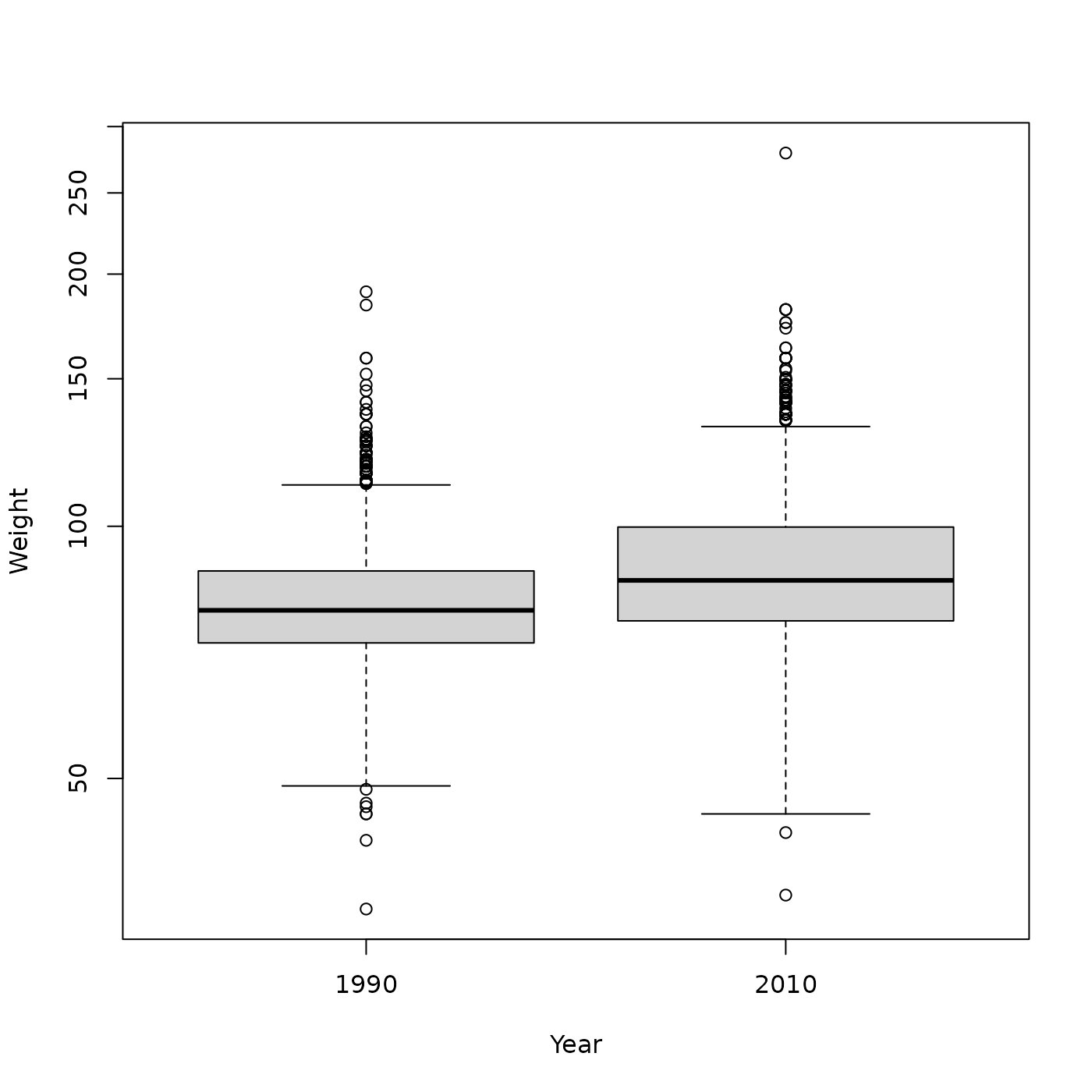
Session information
sessionInfo()
#> R version 4.3.3 (2024-02-29)
#> Platform: x86_64-pc-linux-gnu (64-bit)
#> Running under: Ubuntu 22.04.4 LTS
#>
#> Matrix products: default
#> BLAS:   /usr/lib/x86_64-linux-gnu/openblas-pthread/libblas.so.3
#> LAPACK: /usr/lib/x86_64-linux-gnu/openblas-pthread/libopenblasp-r0.3.20.so;  LAPACK version 3.10.0
#>
#> locale:
#>  [1] LC_CTYPE=C.UTF-8       LC_NUMERIC=C           LC_TIME=C.UTF-8
#>  [4] LC_COLLATE=C.UTF-8     LC_MONETARY=C.UTF-8    LC_MESSAGES=C.UTF-8
#>  [7] LC_PAPER=C.UTF-8       LC_NAME=C              LC_ADDRESS=C
#> [10] LC_TELEPHONE=C         LC_MEASUREMENT=C.UTF-8 LC_IDENTIFICATION=C
#>
#> time zone: UTC
#> tzcode source: system (glibc)
#>
#> attached base packages:
#> [1] stats     graphics  grDevices utils     datasets  methods   base
#>
#> other attached packages:
#> [1] dplyr_1.1.4
#>
#> loaded via a namespace (and not attached):
#>  [1] bit_4.0.5         jsonlite_1.8.8    highr_0.10        compiler_4.3.3
#>  [5] crayon_1.5.2      tidyselect_1.2.1  parallel_4.3.3    jquerylib_0.1.4
#>  [9] systemfonts_1.0.6 textshaping_0.3.7 yaml_2.3.8        fastmap_1.1.1
#> [13] readr_2.1.5       R6_2.5.1          generics_0.1.3    knitr_1.45
#> [17] tibble_3.2.1      desc_1.4.3        bslib_0.6.2       pillar_1.9.0
#> [21] tzdb_0.4.0        rlang_1.1.3       utf8_1.2.4        cachem_1.0.8
#> [25] xfun_0.43         fs_1.6.3          sass_0.4.9        bit64_4.0.5
#> [29] memoise_2.0.1     cli_3.6.2         withr_3.0.0       pkgdown_2.0.7
#> [33] magrittr_2.0.3    digest_0.6.35     vroom_1.6.5       hms_1.1.3
#> [37] lifecycle_1.0.4   vctrs_0.6.5       evaluate_0.23     glue_1.7.0
#> [41] ragg_1.3.0        fansi_1.0.6       rmarkdown_2.26    purrr_1.0.2
#> [45] tools_4.3.3       pkgconfig_2.0.3   htmltools_0.5.8