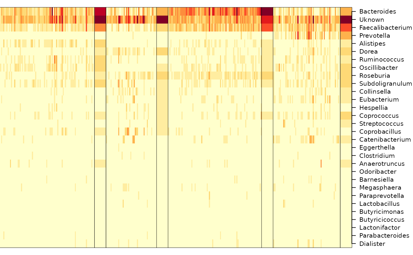
Heatmap representation of samples assigned to Dirichlet components.

Produce a heat map summarizing count data, grouped by Dirichlet component.

Usage

heatmapdmn(count, fit1, fitN, ntaxa = 30, ...,
    transform = sqrt, lblwidth = 0.2 * nrow(count), col = .gradient)

Arguments

count: A matrix of sample x taxon counts, as supplied to dmn.
fit1: An instance of class dmn, from a model fit to a single Dirichlet component, k=1 in dmn.
fitN: An instance of class dmn, from a model fit to N != 1 components, k=N in dmn.
ntaxa: The ntaxa most numerous taxa to display counts for.
...: Additional arguments, ignored.
transform: Transformation to apply to count data prior to visualization; this does not influence mixture membership or taxnomic ordering.
lblwidth: The proportion of the plot to dedicate to taxanomic labels, as a fraction of the number of samples to be plotted.
col: The colors used to display (possibly transformed, by transform) count data, as used by image.

Details

Columns of the heat map correspond to samples. Samples are grouped by Dirichlet component, with average (Dirichlet) components summarized as a separate wide column. Rows correspond to taxonomic groups, ordered based on contribution to Dirichlet components.

Author

Martin Morgan mailto:mtmorgan.xyz@gmail.com

Examples

## counts
fl <- system.file(package="DirichletMultinomial", "extdata",
                  "Twins.csv")
count <- t(as.matrix(read.csv(fl, row.names=1)))

## all and best-fit clustering
data(fit)
lplc <- sapply(fit, laplace)
best <- fit[[which.min(lplc)]]

heatmapdmn(count, fit[[1]], best, 30)