DirichletMultinomial for Clustering and Classification of Microbiome Data

Modified: 6 March 2012, 19 October 2024 (HTML version)

This document illustrates the main features of the DirichletMultinomial package, and in the process replicates key tables and figures from Holmes et al., https://doi.org/10.1371/journal.pone.0030126.

We start by loading the package, in addition to the packages lattice (for visualization) and parallel (for use of multiple cores during cross-validation).

library(DirichletMultinomial)
library(lattice)
library(parallel)

We set the width of R output to 70 characters, and the number of floating point digits displayed to two. The full flag is set to FALSE, so that cached values are used instead of re-computing during production of this vignette. The package defines a set of standard colors; we use .qualitative during visualization.

options(width=70, digits=2)
full <- FALSE
.qualitative <- DirichletMultinomial:::.qualitative

Data

The data used in Homes et al. is included in the package. We read the data in to a matrix count of samples by taxa.

fl <- system.file(package="DirichletMultinomial", "extdata", "Twins.csv")
count <- t(as.matrix(read.csv(fl, row.names=1)))
count[1:5, 1:3]
#>         Acetanaerobacterium Acetivibrio Acetobacterium
#> TS1.2                     0           0              0
#> TS10.2                    0           0              0
#> TS100.2                   0           0              0
#> TS100                     1           0              0
#> TS101.2                   0           0              0

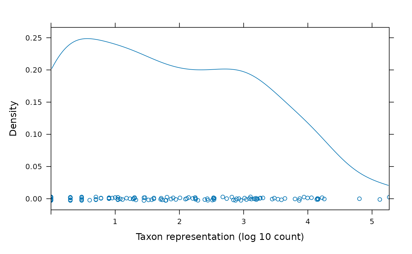
The figure below shows the distribution of reads from each taxon, on a log scale.

cnts <- log10(colSums(count))
densityplot(
    cnts, xlim=range(cnts),
    xlab="Taxon representation (log 10 count)"
)

Clustering

The dmn function fits a Dirichlet-Multinomial model, taking as input the count data and a parameter $k$ representing the number of Dirichlet components to model. Here we fit the count data to values of $k$ from 1 to 7, displaying the result for $k = 4$ . A sense of the model return value is provided by the documentation for the R object fit, class ? DMN.

if (full) {
    fit <- mclapply(1:7, dmn, count=count, verbose=TRUE)
    save(fit, file=file.path(tempdir(), "fit.rda"))
} else data(fit)
fit[[4]]
#> class: DMN 
#> k: 4 
#> samples x taxa: 278 x 130 
#> Laplace: 38781 BIC: 40425 AIC: 39477

The return value can be queried for measures of fit (Laplace, AIC, BIC); these are plotted for different $k$ in The figure. The best fit is for $k=4$ distinct Dirichlet components.

lplc <- sapply(fit, laplace)
plot(lplc, type="b", xlab="Number of Dirichlet Components", ylab="Model Fit")

(best <- fit[[which.min(lplc)]])
#> class: DMN 
#> k: 4 
#> samples x taxa: 278 x 130 
#> Laplace: 38781 BIC: 40425 AIC: 39477

In addition to laplace goodness of fit can be assessed with the AIC and BIC functions.

The mixturewt function reports the weight $\pi$ and homogeneity $\theta$ (large values are more homogeneous) of the fitted model. mixture returns a matrix of sample x estimated Dirichlet components; the argument assign returns a vector of length equal to the number of samples indicating the component with maximum value.

mixturewt(best)
#>     pi theta
#> 1 0.31    52
#> 2 0.17    19
#> 3 0.30    53
#> 4 0.22    30
head(mixture(best), 3)
#>            [,1]    [,2]    [,3]    [,4]
#> TS1.2   1.0e+00 2.1e-11 8.6e-06 3.3e-08
#> TS10.2  3.8e-08 3.3e-04 1.0e+00 2.8e-10
#> TS100.2 7.2e-09 8.8e-01 8.0e-13 1.2e-01

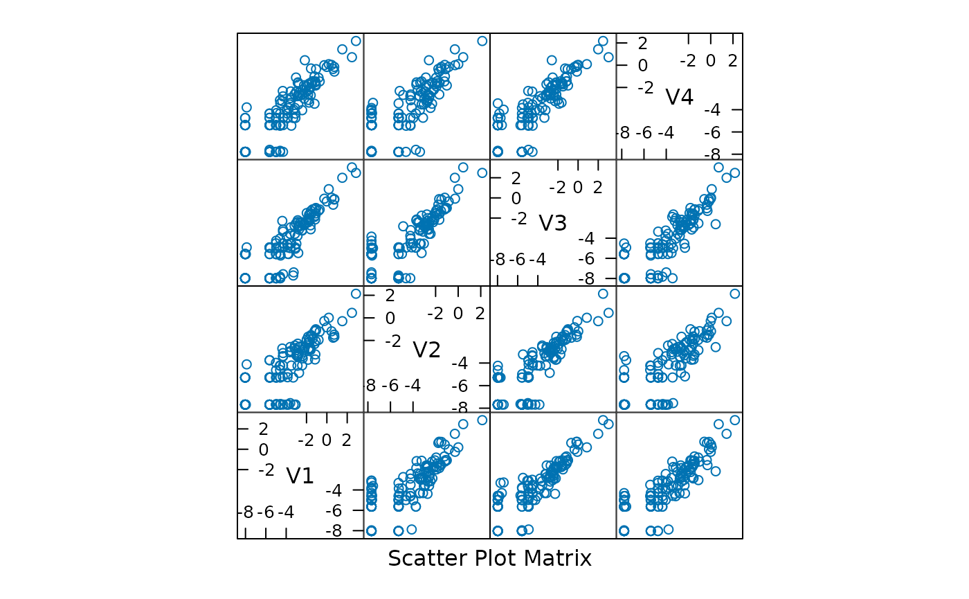
The fitted function describes the contribution of each taxonomic group (each point in the panels of the figure to the Dirichlet components; the diagonal nature of the points in a panel suggest that the Dirichlet components are correlated, perhaps reflecting overall numerical abundance.

splom(log(fitted(best)))

The posterior mean difference between the best and single-component Dirichlet multinomial model measures how each component differs from the population average; the sum is a measure of total difference from the mean.

p0 <- fitted(fit[[1]], scale=TRUE) # scale by theta
p4 <- fitted(best, scale=TRUE)
colnames(p4) <- paste("m", 1:4, sep="")
(meandiff <- colSums(abs(p4 - as.vector(p0))))
#>   m1   m2   m3   m4 
#> 0.26 0.47 0.51 0.34
sum(meandiff)
#> [1] 1.6

The table below summarizes taxonomic contributions to each Dirichlet component.

diff <- rowSums(abs(p4 - as.vector(p0)))
o <- order(diff, decreasing=TRUE)
cdiff <- cumsum(diff[o]) / sum(diff)
df <- cbind(Mean=p0[o], p4[o,], diff=diff[o], cdiff)
DT::datatable(df) |>
    DT::formatRound(colnames(df), digits = 4)

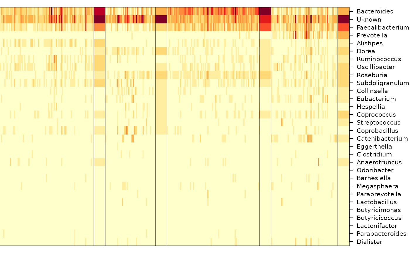
The figure shows samples arranged by Dirichlet component, with samples placed into the component for which they had the largest fitted value.

heatmapdmn(count, fit[[1]], best, 30)

Generative classifier

The following reads in phenotypic information (‘Lean’, ‘Obese’, ‘Overweight’) for each sample.

fl <- system.file(package="DirichletMultinomial", "extdata", "TwinStudy.t")
pheno0 <- scan(fl)
lvls <- c("Lean", "Obese", "Overwt")
pheno <- factor(lvls[pheno0 + 1], levels=lvls)
names(pheno) <- rownames(count)
table(pheno)
#> pheno
#>   Lean  Obese Overwt 
#>     61    193     24

Here we subset the count data into sub-counts, one for each phenotype. We retain only the Lean and Obese groups for subsequent analysis.

counts <- lapply(levels(pheno), csubset, count, pheno)
sapply(counts, dim)
#>      [,1] [,2] [,3]
#> [1,]   61  193   24
#> [2,]  130  130  130
keep <- c("Lean", "Obese")
count <- count[pheno %in% keep,]
pheno <- factor(pheno[pheno %in% keep], levels=keep)

The dmngroup function identifies the best (minimum Laplace score) Dirichlet-multinomial model for each group.

if (full) {
    bestgrp <- dmngroup(
        count, pheno, k=1:5, verbose=TRUE, mc.preschedule=FALSE
    )
    save(bestgrp, file=file.path(tempdir(), "bestgrp.rda"))
} else data(bestgrp)

The Lean group is described by a model with one component, the Obese group by a model with three components. Three of the four Dirichlet components of the original single group (best) model are represented in the Obese group, the other in the Lean group. The total Laplace score of the two group model is less than of the single-group model, indicating information gain from considering groups separately.

bestgrp
#> class: DMNGroup 
#> summary:
#>       k samples taxa   NLE LogDet Laplace   BIC   AIC
#> Lean  1      61  130  9066    162    9027  9333  9196
#> Obese 3     193  130 26770    407   26613 27801 27162
lapply(bestgrp, mixturewt)
#> $Lean
#>   pi theta
#> 1  1    35
#> 
#> $Obese
#>     pi theta
#> 1 0.53    45
#> 2 0.26    33
#> 3 0.22    18
c(
    sapply(bestgrp, laplace),
    'Lean+Obese' = sum(sapply(bestgrp, laplace)),
    Single = laplace(best)
)
#>       Lean      Obese Lean+Obese     Single 
#>       9027      26613      35641      38781

The predict function assigns samples to classes; the confusion matrix shows that the classifier is moderately effective.

xtabs(~pheno + predict(bestgrp, count, assign=TRUE))
#>        predict(bestgrp, count, assign = TRUE)
#> pheno   Lean Obese
#>   Lean    38    23
#>   Obese   15   178

The cvdmngroup function performs cross-validation. This is a computationally expensive step.

if (full) {
    ## full leave-one-out; expensive!
    xval <- cvdmngroup(
        nrow(count), count, c(Lean=1, Obese=3), pheno,
        verbose=TRUE, mc.preschedule=FALSE
    )
    save(xval, file=file.path(tempdir(), "xval.rda"))
} else data(xval)

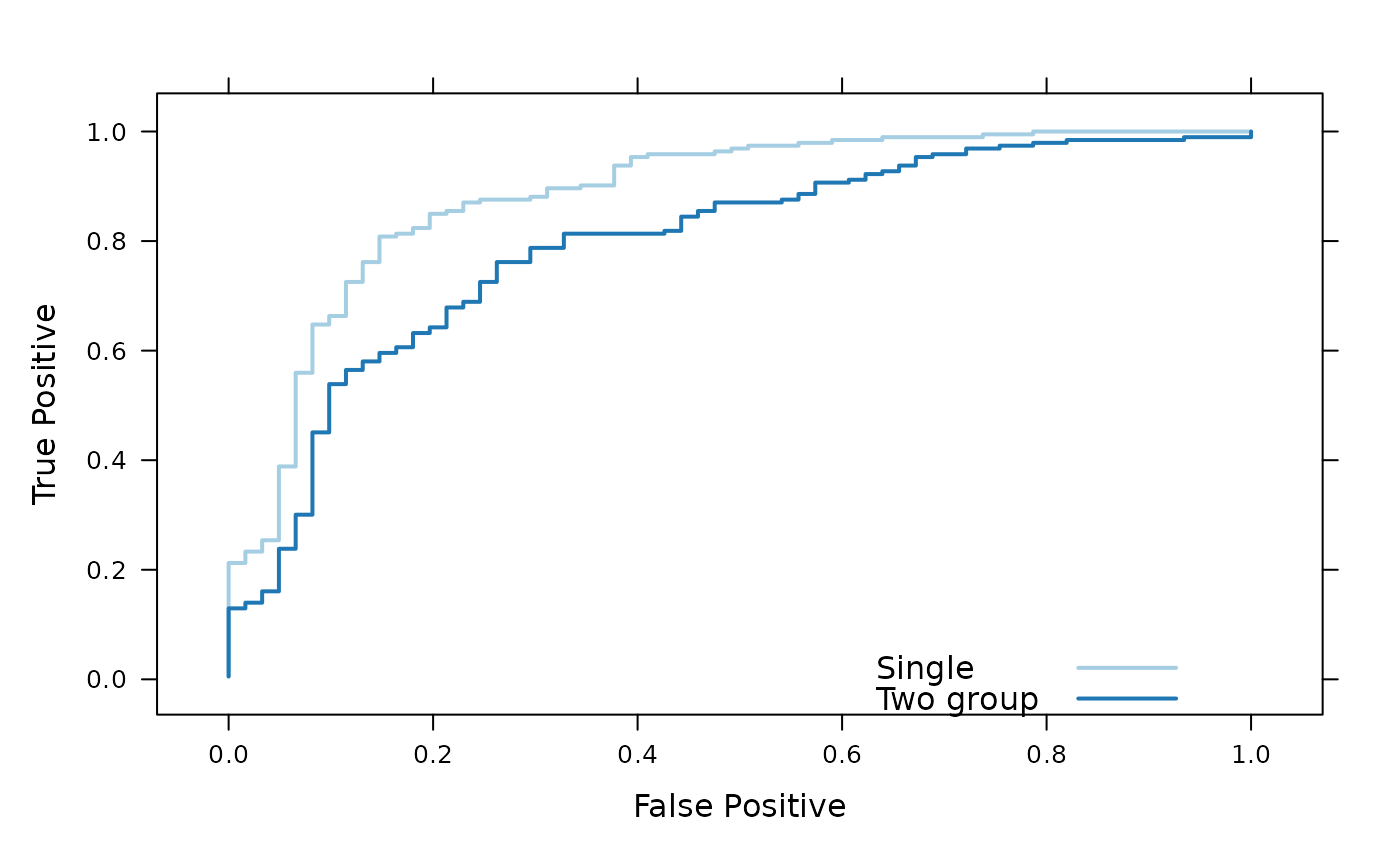
The figure shows an ROC curve for the single and two-group classifier. The single group classifier is performing better than the two-group classifier.

bst <- roc(pheno[rownames(count)] == "Obese",
predict(bestgrp, count)[,"Obese"])
bst$Label <- "Single"
two <- roc(pheno[rownames(xval)] == "Obese", xval[,"Obese"])
two$Label <- "Two group"
both <- rbind(bst, two)
pars <- list(superpose.line=list(col=.qualitative[1:2], lwd=2))
xyplot(
    TruePostive ~ FalsePositive, group=Label, both,
    type="l", par.settings=pars,
    auto.key=list(lines=TRUE, points=FALSE, x=.6, y=.1),
    xlab="False Positive", ylab="True Positive"
)

sessionInfo()
#> R version 4.4.1 (2024-06-14)
#> Platform: x86_64-pc-linux-gnu
#> Running under: Ubuntu 22.04.5 LTS
#> 
#> Matrix products: default
#> BLAS:   /usr/lib/x86_64-linux-gnu/openblas-pthread/libblas.so.3 
#> LAPACK: /usr/lib/x86_64-linux-gnu/openblas-pthread/libopenblasp-r0.3.20.so;  LAPACK version 3.10.0
#> 
#> locale:
#>  [1] LC_CTYPE=C.UTF-8       LC_NUMERIC=C          
#>  [3] LC_TIME=C.UTF-8        LC_COLLATE=C.UTF-8    
#>  [5] LC_MONETARY=C.UTF-8    LC_MESSAGES=C.UTF-8   
#>  [7] LC_PAPER=C.UTF-8       LC_NAME=C             
#>  [9] LC_ADDRESS=C           LC_TELEPHONE=C        
#> [11] LC_MEASUREMENT=C.UTF-8 LC_IDENTIFICATION=C   
#> 
#> time zone: UTC
#> tzcode source: system (glibc)
#> 
#> attached base packages:
#> [1] parallel  stats4    stats     graphics  grDevices utils    
#> [7] datasets  methods   base     
#> 
#> other attached packages:
#> [1] lattice_0.22-6              DirichletMultinomial_1.47.2
#> [3] IRanges_2.38.1              S4Vectors_0.42.1           
#> [5] BiocGenerics_0.50.0         BiocStyle_2.32.1           
#> 
#> loaded via a namespace (and not attached):
#>  [1] cli_3.6.3           knitr_1.48          rlang_1.1.4        
#>  [4] xfun_0.48           highr_0.11          textshaping_0.4.0  
#>  [7] jsonlite_1.8.9      DT_0.33             htmltools_0.5.8.1  
#> [10] ragg_1.3.3          sass_0.4.9          rmarkdown_2.28     
#> [13] grid_4.4.1          crosstalk_1.2.1     evaluate_1.0.1     
#> [16] jquerylib_0.1.4     fastmap_1.2.0       yaml_2.3.10        
#> [19] lifecycle_1.0.4     bookdown_0.41       BiocManager_1.30.25
#> [22] compiler_4.4.1      fs_1.6.4            htmlwidgets_1.6.4  
#> [25] systemfonts_1.1.0   digest_0.6.37       R6_2.5.1           
#> [28] magrittr_2.0.3      bslib_0.8.0         tools_4.4.1        
#> [31] pkgdown_2.1.1       cachem_1.1.0        desc_1.4.3

Martin Morgan

19 October 2024

Data

Clustering

Generative classifier