A. Introduction to R • HCABiocTraining

Essential R

A simple calculator

1 + 1
## [1] 2

‘Vectors’ as building blocks

c(1, 2, 3)
## [1] 1 2 3
c("January", "February", "March")
## [1] "January"  "February" "March"
c(TRUE, FALSE)
## [1]  TRUE FALSE

Variables, missing values and ‘factors’

age <- c(27, NA, 32, 29)
gender <- factor(
    c("Female", "Male", "Non-binary", NA),
    levels = c("Female", "Male", "Non-binary")
)

Data structures to coordinate related vectors – the data.frame

df <- data.frame(
    age = c(27, NA, 32, 29),
    gender = gender
)
df
##   age     gender
## 1  27     Female
## 2  NA       Male
## 3  32 Non-binary
## 4  29       <NA>

Key opererations on data.frame

df[1:3, c("gender", "age")] – subset on rows and columns
df[["age"]], df$age – select columns

Functions

rnorm(5)        # 5 random normal deviates
## [1]  2.79022372 -0.38764450 -0.23800823  2.07697779 -0.04142712
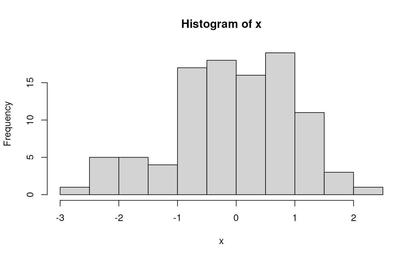
x <- rnorm(100) # 100 random normal deviates
hist(x)         # histogram, approximately normal

plot(density(x)) # a little more sophisticated?

‘Vectorized’ operations, e.g., element-wise addition without an explicit ‘for’ loop

y <- x + rnorm(100)
plot(y ~ x)
fit <- lm(y ~ x)
fit         # an R 'object' containing information about the
## 
## Call:
## lm(formula = y ~ x)
## 
## Coefficients:
## (Intercept)            x  
##     -0.1138       0.9889
            # regression of y on x
abline(fit) # plot points and fitted regression line

anova(fit)  # statistical summary of linear regression
## Analysis of Variance Table
## 
## Response: y
##           Df  Sum Sq Mean Sq F value    Pr(>F)    
## x          1 107.594 107.594   126.5 < 2.2e-16 ***
## Residuals 98  83.351   0.851                      
## ---
## Signif. codes:  0 '***' 0.001 '**' 0.01 '*' 0.05 '.' 0.1 ' ' 1

Write your own functions

hello <- function(who) {
    paste("hello", who, "with", nchar(who), "letters in your name")
}
hello("Martin")
## [1] "hello Martin with 6 letters in your name"

Iterate, usually with lapply() although for() is available

names <- c("Martin", "Thomas")
lapply(names, hello)
## [[1]]
## [1] "hello Martin with 6 letters in your name"
## 
## [[2]]
## [1] "hello Thomas with 6 letters in your name"

Packages

Extend functionality of base R. Can be part of the ‘base’ distribution…

## iterate over the numbers 1 through 8, 'sleeping' for 1 second
## each. Takes about 8 seconds...
system.time({
    lapply(1:8, function(i) Sys.sleep(1))
})
##    user  system elapsed 
##   0.003   0.001   8.011

## sleep in parallel -- takes only 2 seconds
library(parallel)
cl <- makeCluster(4) # cluster of 4 workers
system.time({
    parLapply(cl, 1:8, function(i) Sys.sleep(1))
})
##    user  system elapsed 
##   0.003   0.000   2.089

Tidyverse

The dplyr package introduces the ‘tidyverse’

library(dplyr)

A ‘tibble’ is like a ‘data.frame’, but more user-friendly

tbl <- tibble(
    x = rnorm(100),
    y = x + rnorm(100)
)

## e.g., only displays the first 10 rows
tbl
## # A tibble: 100 × 2
##         x      y
##     <dbl>  <dbl>
##  1  0.579  1.74 
##  2  0.302 -0.214
##  3 -1.51  -2.21 
##  4  0.732  0.980
##  5 -1.11  -2.42 
##  6  1.36   2.63 
##  7 -0.443 -0.989
##  8 -0.391 -0.436
##  9 -1.17  -2.56 
## 10 -1.48  -1.72 
## # … with 90 more rows

The tidyverse makes use of ‘pipes’ |> (the older syntax is %>%). A pipe takes the left-hand side and pass through to the right-hand side. Key dplyr ‘verbs’ can be piped together

filter() rows
select() columns
mutate() to change values
group_by() operate on groups of rows
left_join() (and friends) for joining tibbles based on shared columns

tbl |>
    ## e.g., just rows with non-negative values of x and y
    filter(x > 0, y > 0) |>
    ## add a column
    mutate(distance_from_origin = sqrt(x^2 + y^2))
## # A tibble: 28 × 3
##        x     y distance_from_origin
##    <dbl> <dbl>                <dbl>
##  1 0.579 1.74                 1.83 
##  2 0.732 0.980                1.22 
##  3 1.36  2.63                 2.96 
##  4 0.997 1.38                 1.71 
##  5 1.05  0.974                1.43 
##  6 0.195 0.416                0.459
##  7 0.208 0.305                0.369
##  8 0.298 0.819                0.871
##  9 1.24  2.07                 2.42 
## 10 0.499 0.884                1.02 
## # … with 18 more rows

Visualization

Another example of a contributed package is ggplot2 for visualization

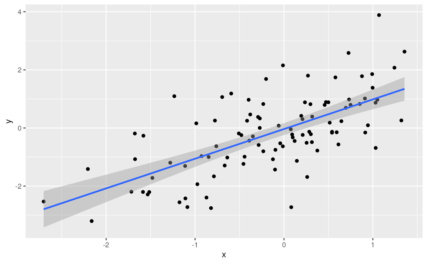
library(ggplot2)
ggplot(tbl) +
    aes(x, y) +                # use 'x' and 'y' columns for plotting...
    geom_point() +             # ...plot points...
    geom_smooth(method = "lm") # ...linear regresion
## `geom_smooth()` using formula = 'y ~ x'

Where do Packages Come From?

CRAN: Comprehensive R Archive Network. More than 18,000 packages. Some help from CRAN Task Views in identifying relevant packages.
Bioconductor: More than 2100 packages relevant to high-throughput genomic analysis. Vignettes are an important part of Bioconductor packages.

Install packages once per R installation, using BiocManager::install(<package-name>) (CRAN or Bioconductor)

What about GitHub? Packages haven’t been checked by a formal system, so may have incomplete code, documentation, dependencies on other packages, etc. Authors may not yet be committed to long-term maintenance of their package.

Help & Vignettes

Help pages, e.g., ?lm

Vignettes, e.g.,

vignette(package = "ggplot2")
vignette("ggplot2-specs", "ggplot2")

Google, StackOverflow, etc…