D. Using Single-Cell Data into Bioconductor Work Flows
d-objects.RmdThis article explores more direct manipulation of single cell objects
and their integration into Seurat, R and
Bioconductor work flows. We illustrate the basics of object
manipulation provided by existing packages, and then hint at how one
might start to work with data ‘outside the box’ provided by these
packages. This can be important for both routine (e.g., creating a
subset of data based on gene set membership) or advanced (e.g.,
implementing a new analysis method) tasks. The focus is on
Bioconductor’s SingleCellExperiment object becuase
of the rich supporting infastructure (e.g., annotation resources or the
powerful GenomicRanges
infrastructure) within Bioconductor; similar operations can
also be accomplished with the Seurat object.
We start by loading packages we’ll use today.
library(HCABiocTraining)

## single cell data representation in R
library(Seurat)               # Seurat representation
library(SingleCellExperiment) # Bioconductor representation

## data access
library(cellxgenedp)

## general programming tools
library(dplyr)
library(ggplot2)
library(plotly)
We illustrate these steps with data from CELLxGENE retrieved in the previous article. For our own data we would need to proceed from a simple count matrix produced by Cell Ranger (etc.) through careful quality control, normalization, data integration / batch coorrection, etc., as illustrated in a different article.
Exploring Objects
Seurat
Based on Getting Started with Seurat and the Seurat - Guided Clustering Tutorial.
Retrieve the Seurat object
## use a known dataset ID, discovered previously..
dataset <- "de985818-285f-4f59-9dbd-d74968fddba3"
training_cxg_dataset(dataset)
## title: A single-cell atlas of the healthy breast tissues reveals
##     clinically relevant clusters of breast epithelial cells
## description: Single-cell RNA sequencing (scRNA-seq) is an evolving
##     technology used to elucidate the cellular architecture of adult
##     organs. Previous scRNA-seq on breast tissue utilized reduction
##     mammoplasty samples, which are often histologically abnormal. We
##     report a rapid tissue collection/processing protocol to perform
##     scRNA-seq of breast biopsies of healthy women and identify 23
##     breast epithelial cell clusters. Putative cell-of-origin signatures
##     derived from these clusters are applied to analyze transcriptomes
##     of ~3,000 breast cancers. Gene signatures derived from mature
##     luminal cell clusters are enriched in ~68% of breast cancers,
##     whereas a signature from a luminal progenitor cluster is enriched
##     in ~20% of breast cancers. Overexpression of luminal progenitor
##     cluster-derived signatures in HER2+, but not in other subtypes, is
##     associated with unfavorable outcome. We identify TBX3 and PDK4 as
##     genes co-expressed with estrogen receptor (ER) in the normal
##     breasts, and their expression analyses in >550 breast cancers
##     enable prognostically relevant subclassification of ER+ breast
##     cancers.
## authors: Bhat-Nakshatri, Poornima; Gao, Hongyu; Sheng, Liu; McGuire,
##     Patrick C.; Xuei, Xiaoling; Wan, Jun; Liu, Yunlong; Althouse,
##     Sandra K.; Colter, Austyn; Sandusky, George; Storniolo, Anna Maria;
##     Nakshatri, Harikrishna
## journal: Cell Reports Medicine
## assays: 10x 3' v2; 10x 3' v3
## organism: Homo sapiens
## ethnicity: African American; Chinese; European

## download (or retieve from the local cache) the file
seurat_file <-
    files() |>
    dplyr::filter(filetype == "RDS", dataset_id == dataset) |>
    files_download(dry.run = FALSE)

seurat <- readRDS(seurat_file)
Retrieve the annotation on each cell using [[]],
e.g.,
seurat[[]] |>
    as_tibble() |>
    dplyr::count(self_reported_ethnicity)
## # A tibble: 3 × 2
##   self_reported_ethnicity     n
##   <fct>                   <int>
## 1 European                21725
## 2 Chinese                  7454
## 3 African American         2517

seurat[[]] |>
    as_tibble() |>
    dplyr::count(cell_type)
## # A tibble: 6 × 2
##   cell_type                                    n
##   <fct>                                    <int>
## 1 endocrine cell                              64
## 2 B cell                                     215
## 3 basal cell                                7040
## 4 endothelial cell of lymphatic vessel       133
## 5 luminal epithelial cell of mammary gland  4257
## 6 progenitor cell                          19987
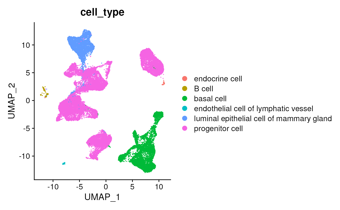
Recreate a simple UMAP
UMAPPlot(seurat, group.by = "cell_type")
I remove the seurat object from the session, in hopes of
freeing up a bit of memory.
rm(seurat)SingleCellExperiment
Retreive the .h5ad file
## download (or retieve from the local cache) the file
dataset <- "de985818-285f-4f59-9dbd-d74968fddba3"
h5ad_file <-
    files() |>
    dplyr::filter(filetype == "H5AD", dataset_id == dataset) |>
    files_download(dry.run = FALSE)

## import into R as a SingleCellExperiment
h5ad <- training_read_h5ad_as_sce(h5ad_file)
Basic Manipulation
The following is based on Orchestrating Single-Cell Analysis with Bioconductor. This resource is separated into introductory, basic, advanced, and multi-sample sections, with a collection of workflows illustrating use. A good place to start is with a workflow to get a feel for data analysis, and then to refer back to earlier sections for more detailed operations or understanding.
Displaying the SingleCellExperiment…
h5ad
## class: SingleCellExperiment
## dim: 33234 31696
## metadata(3): default_embedding schema_version title
## assays(1): counts
## rownames(33234): ENSG00000243485 ENSG00000237613 ... ENSG00000277475
##   ENSG00000268674
## rowData names(4): feature_is_filtered feature_name feature_reference
##   feature_biotype
## colnames(31696): CMGpool_AAACCCAAGGACAACC CMGpool_AAACCCACAATCTCTT ...
##   K109064_TTTGTTGGTTGCATCA K109064_TTTGTTGGTTGGACCC
## colData names(34): donor_id self_reported_ethnicity_ontology_term_id
##   ... self_reported_ethnicity development_stage
## reducedDimNames(3): X_pca X_tsne X_umap
## mainExpName: NULL
## altExpNames(0):
…suggests the data available and how to access it – there are 33234
genes and 31696 cells. The ‘raw’ data include a gene x cell count
matricies (assay()) with annotations on the genes
(rowData()) and columns (cellData()), and with
reduced-dimension summaries.
For instance, the cell (column) annotations are easily accessible and summarized as
colData(h5ad) |>
    as_tibble()
## # A tibble: 31,696 × 34
##    donor_id      self_…¹ donor…² donor…³ famil…⁴ organ…⁵ tyrer…⁶ sampl…⁷ sampl…⁸
##    <fct>         <fct>   <fct>   <fct>   <fct>   <fct>   <fct>   <fct>   <fct>
##  1 pooled [D9,D… HANCES… pooled… pooled… pooled… NCBITa… pooled… pooled… cryopr…
##  2 pooled [D9,D… HANCES… pooled… pooled… pooled… NCBITa… pooled… pooled… cryopr…
##  3 pooled [D9,D… HANCES… pooled… pooled… pooled… NCBITa… pooled… pooled… cryopr…
##  4 pooled [D9,D… HANCES… pooled… pooled… pooled… NCBITa… pooled… pooled… cryopr…
##  5 pooled [D9,D… HANCES… pooled… pooled… pooled… NCBITa… pooled… pooled… cryopr…
##  6 pooled [D9,D… HANCES… pooled… pooled… pooled… NCBITa… pooled… pooled… cryopr…
##  7 pooled [D9,D… HANCES… pooled… pooled… pooled… NCBITa… pooled… pooled… cryopr…
##  8 pooled [D9,D… HANCES… pooled… pooled… pooled… NCBITa… pooled… pooled… cryopr…
##  9 pooled [D9,D… HANCES… pooled… pooled… pooled… NCBITa… pooled… pooled… cryopr…
## 10 pooled [D9,D… HANCES… pooled… pooled… pooled… NCBITa… pooled… pooled… cryopr…
## # … with 31,686 more rows, 25 more variables: tissue_ontology_term_id <fct>,
## #   development_stage_ontology_term_id <fct>, suspension_uuid <fct>,
## #   suspension_type <fct>, library_uuid <fct>, assay_ontology_term_id <fct>,
## #   mapped_reference_annotation <fct>, is_primary_data <lgl>,
## #   cell_type_ontology_term_id <fct>, author_cell_type <fct>,
## #   disease_ontology_term_id <fct>, sex_ontology_term_id <fct>,
## #   nCount_RNA <dbl>, nFeature_RNA <int>, percent.mito <dbl>, …
colData(h5ad) |>
    as_tibble() |>
    group_by(donor_id, self_reported_ethnicity) |>
    dplyr::count()
## # A tibble: 7 × 3
## # Groups:   donor_id, self_reported_ethnicity [7]
##   donor_id                 self_reported_ethnicity     n
##   <fct>                    <fct>                   <int>
## 1 D1                       European                 2303
## 2 D2                       European                  864
## 3 D3                       African American         2517
## 4 D4                       European                 1771
## 5 D5                       European                 2244
## 6 D11                      Chinese                  7454
## 7 pooled [D9,D7,D8,D10,D6] European                14543
colData(h5ad) |>
    as_tibble() |>
    dplyr::count(cell_type, sort = TRUE)
## # A tibble: 6 × 2
##   cell_type                                    n
##   <fct>                                    <int>
## 1 progenitor cell                          19987
## 2 basal cell                                7040
## 3 luminal epithelial cell of mammary gland  4257
## 4 B cell                                     215
## 5 endothelial cell of lymphatic vessel       133
## 6 endocrine cell                              64
Many common operations have been standardized in a number of
Bioconductor packages. For instance, use functionality from the
scater package to
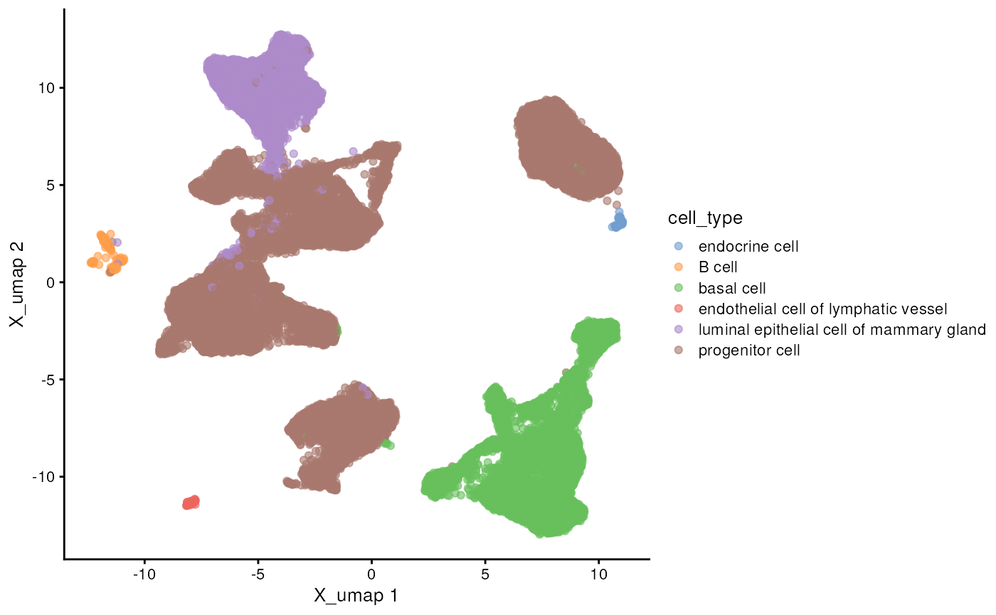
visualize the UMAP present in the object, coloring by the
cell_type column data annotation.
scater::plotReducedDim(h5ad, "X_umap", color_by = "cell_type")
Outside the Box
This section uses the SingleCellExperiment; similar operations can be performed on Seurat objects.
It very easy to find out information about the samples included in the study, e.g., the individual donors, their ethnicty, and family history of breast cancer (the specific information available depends on the data submitted by the original investigator).
colData(h5ad) |>
as_tibble() |>
dplyr::count(
donor_id, self_reported_ethnicity, family_history_breast_cancer
)
## # A tibble: 7 × 4
## donor_id self_reported_ethnicity family_history_breast…¹ n
## <fct> <fct> <fct> <int>
## 1 D1 European unknown 2303
## 2 D2 European True 864
## 3 D3 African American True 2517
## 4 D4 European False 1771
## 5 D5 European True 2244
## 6 D11 Chinese True 7454
## 7 pooled [D9,D7,D8,D10,D6] European pooled [unknown,False,… 14543
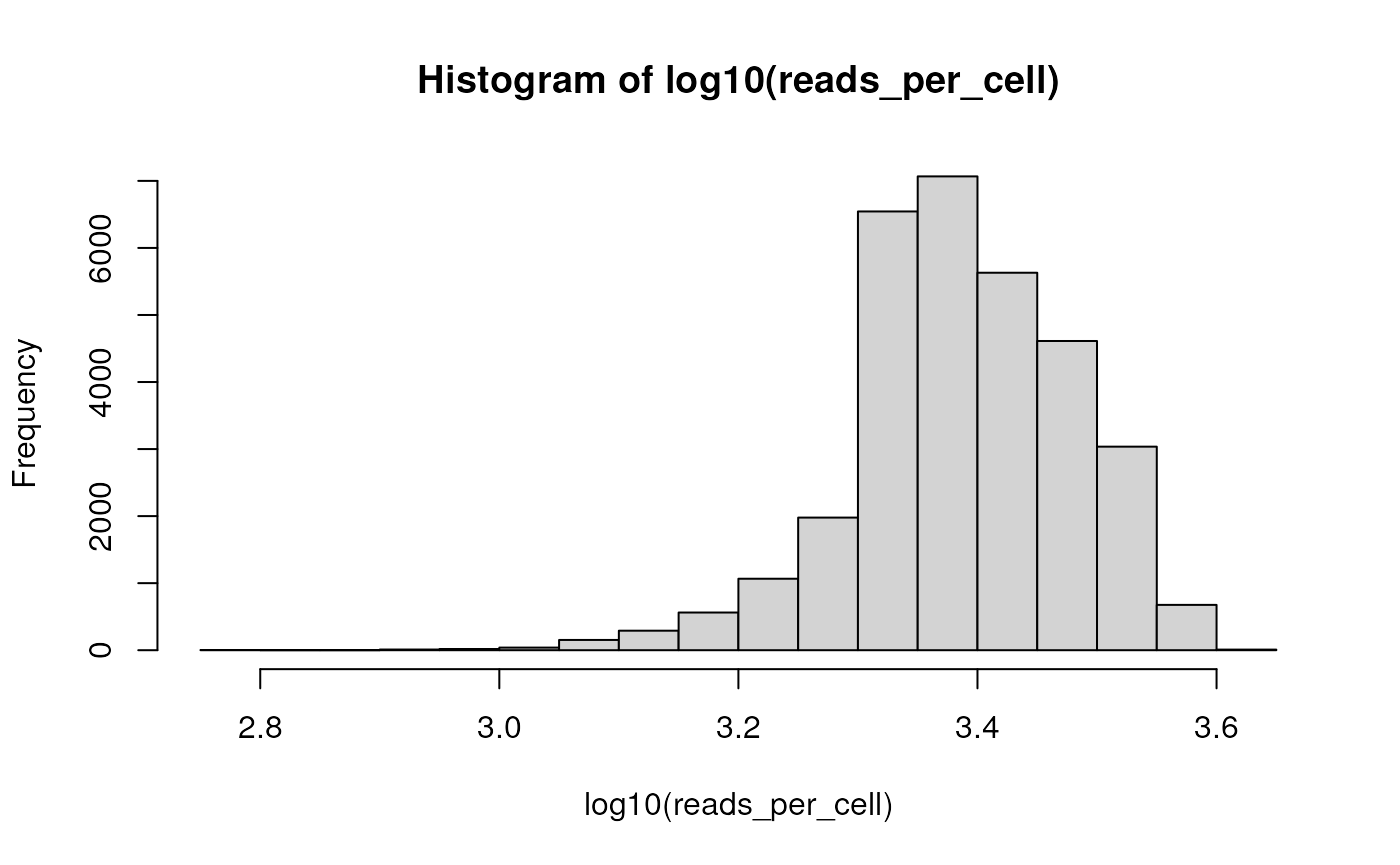
## # … with abbreviated variable name ¹family_history_breast_cancerThe actual feature x sample counts are available and easily manipulated, as illustrated by this plot of the distribution of reads per cell…
reads_per_cell <-
    h5ad |>
    ## retrieve the matrix of gene x cell counts
    assay("counts", withDimnames = FALSE) |>
    ## calculate the column sums, i.e., reads mapped to each cell
    colSums()

hist(log10(reads_per_cell))
…or to remove genes with non-zero counts
reads_per_gene <-
    h5ad |>
    assay("counts", withDimnames = FALSE) |>
    rowSums()

table(reads_per_gene != 0)
##
## FALSE  TRUE
## 10499 22735

h5ad[reads_per_gene != 0,]
## class: SingleCellExperiment
## dim: 22735 31696
## metadata(3): default_embedding schema_version title
## assays(1): counts
## rownames(22735): ENSG00000238009 ENSG00000237491 ... ENSG00000276345
##   ENSG00000271254
## rowData names(4): feature_is_filtered feature_name feature_reference
##   feature_biotype
## colnames(31696): CMGpool_AAACCCAAGGACAACC CMGpool_AAACCCACAATCTCTT ...
##   K109064_TTTGTTGGTTGCATCA K109064_TTTGTTGGTTGGACCC
## colData names(34): donor_id self_reported_ethnicity_ontology_term_id
##   ... self_reported_ethnicity development_stage
## reducedDimNames(3): X_pca X_tsne X_umap
## mainExpName: NULL
## altExpNames(0):
Visualization
The previous section created a static visualization from the ‘UMAP’
reduced dimension representation using
scater::plotReducedDim():
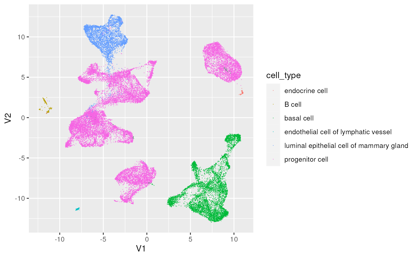
It can be helpful to do this ‘by hand’ to illustrate how one can work directly with SingleCellExperiment objects. First load ggplot2
Then create a tibble containing information about the UMAP, as well as cell (column) annotations
umap <-
    as_tibble(SingleCellExperiment::reducedDim(h5ad, "X_umap")) |>
    bind_cols(
        cell_type = h5ad$cell_type,
        donor_id = h5ad$donor_id,
        self_reported_ethnicity = h5ad$self_reported_ethnicity,
        colname = colnames(h5ad) # unique identifier
    )
## Warning: The `x` argument of `as_tibble.matrix()` must have unique column names if
## `.name_repair` is omitted as of tibble 2.0.0.
## ℹ Using compatibility `.name_repair`.
Visualize the two-dimensional UMAP summary, coloring by cell type
ggplot(umap) +
    aes(x = V1, y = V2, color = cell_type) +
    geom_point(pch = ".")
The plotly package provides a very convenient way to make this an interactive plot
library(plotly)

plot_ly(
    umap,
    x = ~ V1, y =  ~ V2, color = ~ cell_type,
    type = "scatter", mode = "markers", opacity = .8,
    marker = list(symbol = "circle-open", line = list(width = 1))
) |> toWebGL() # using webGL greatly speeds display!
A suprisingly straight-forward (but admittedly advanced) helper function uses shiny to allows us to write an application to select data we are interested in… check it out!
result <- training_cell_viewer(umap) # select some cells of interest
result
## subset the SingleCellExperiment to just those cells
h5ad[, result$colname]
Gene Sets
The single cell assay detected expression of 33234 genes, but we may often be interested in only a set of these. Such gene sets might be defined by our own research interests, or may be defined as ‘community standards’.
Check out MSigDB – a collection of gene sets! Focus on the Halmarks of Cancer gene sets ‘H: hallmark gene sets’. NOTE MSigDB requires registration, which is triggered by downloading a gene set manually; do that first, even though we use automatically downloaded gene sets.
The helper function training_hallmarks() downloads the
‘Hallmarks of Cancer’ gene sets from MSigDb, translating the ‘Entrez’
gene identifiers in the gene sets to the ‘Ensembl’ identifiers
(rownames(h5ad)) in our data.
hallmarks <- training_hallmarks()
## visit 'https://www.gsea-msigdb.org/gsea/msigdb/human/collections.jsp'
##     to register for use of the MSigDb 'hallmarks' dataset.
## 'select()' returned 1:many mapping between keys and columns
hallmarks
## # A tibble: 8,220 × 3
##    gene            set                                      description
##    <chr>           <chr>                                    <chr>
##  1 ENSG00000000938 HALLMARK_ALLOGRAFT_REJECTION             http://www.gsea-msi…
##  2 ENSG00000000971 HALLMARK_INTERFERON_GAMMA_RESPONSE       http://www.gsea-msi…
##  3 ENSG00000000971 HALLMARK_COMPLEMENT                      http://www.gsea-msi…
##  4 ENSG00000000971 HALLMARK_COAGULATION                     http://www.gsea-msi…
##  5 ENSG00000000971 HALLMARK_KRAS_SIGNALING_UP               http://www.gsea-msi…
##  6 ENSG00000001084 HALLMARK_MTORC1_SIGNALING                http://www.gsea-msi…
##  7 ENSG00000001084 HALLMARK_XENOBIOTIC_METABOLISM           http://www.gsea-msi…
##  8 ENSG00000001084 HALLMARK_GLYCOLYSIS                      http://www.gsea-msi…
##  9 ENSG00000001084 HALLMARK_REACTIVE_OXYGEN_SPECIES_PATHWAY http://www.gsea-msi…
## 10 ENSG00000001084 HALLMARK_HEME_METABOLISM                 http://www.gsea-msi…
## # … with 8,210 more rows

## gene sets and their counts
hallmarks |> dplyr::count(set)
## # A tibble: 50 × 2
##    set                                  n
##    <chr>                            <int>
##  1 HALLMARK_ADIPOGENESIS              210
##  2 HALLMARK_ALLOGRAFT_REJECTION       343
##  3 HALLMARK_ANDROGEN_RESPONSE         104
##  4 HALLMARK_ANGIOGENESIS               36
##  5 HALLMARK_APICAL_JUNCTION           231
##  6 HALLMARK_APICAL_SURFACE             46
##  7 HALLMARK_APOPTOSIS                 182
##  8 HALLMARK_BILE_ACID_METABOLISM      114
##  9 HALLMARK_CHOLESTEROL_HOMEOSTASIS    77
## 10 HALLMARK_COAGULATION               160
## # … with 40 more rows
Suppose we are interested in the HALLMARK_P53_PATHWAY
gene set
We can create a subset of our data with just these genes (some
identifiers in p53_gene_set are not present in our observed
data…)
p53_rows <- rownames(h5ad) %in% pull(p53_gene_set, "gene")
h5ad_p53 <- h5ad[p53_rows,]
h5ad_p53
## class: SingleCellExperiment
## dim: 200 31696
## metadata(3): default_embedding schema_version title
## assays(1): counts
## rownames(200): ENSG00000116213 ENSG00000142627 ... ENSG00000142192
##   ENSG00000160310
## rowData names(4): feature_is_filtered feature_name feature_reference
##   feature_biotype
## colnames(31696): CMGpool_AAACCCAAGGACAACC CMGpool_AAACCCACAATCTCTT ...
##   K109064_TTTGTTGGTTGCATCA K109064_TTTGTTGGTTGGACCC
## colData names(34): donor_id self_reported_ethnicity_ontology_term_id
##   ... self_reported_ethnicity development_stage
## reducedDimNames(3): X_pca X_tsne X_umap
## mainExpName: NULL
## altExpNames(0):
These steps illustrate some of the straight-forward ways of integrating scRNASeq analysis into larger bioinformatic work flows.