Day 2: Data Management, Visualization, and Analysis

Log on to https://ondemand.ccr.buffalo.edu

Set up RStudio for today

source('/projects/rpci/rplect/Rpg520/Rsetdirs.R')

Let RStudio know about your new working directory

Introduction

We use two case studies today. The studies are used to illustrate the data manipulation and statistical analysis tasks that one might expect in day-to-day wet- or dry-lab work in computational oncology.

US CDC Behavioral Risk Factor Surveillance System survey data

We use data from the US Center for Disease Control’s Behavioral Risk Factor Surveillance System (BRFSS) annual survey. Check out the web page for a little more information. We are using a small subset of this data, including a random sample of 20000 observations from each of 1990 and 2010.

In this first case study, We will use functions from the dplyr package to manage our data. dplyr is is a key package in a particular approach to data management in R called the ‘tidyverse’. Tidy analysis uses a standard data structure (a tibble) and relatively small number functions to provide an effective way to accomplish many tasks.

Start by loading the dplyr package.

library(dplyr)

Functions for ‘tidy’ data management include:

filter() – filter data to contain specific rows.
select() – select a subset of columns.
mutate() – change or add columns.

Example functions to summarize data:

count() – simple count of entries in each column.
summarize() – e.g., mean() or var()iance of one or more columns.
group_by() – summarize data by group.

tidyr and other packages complement basic functionality

tidyr::pivot_wider() – change a ‘long’ table to a ‘wide’ table. See example below.

We will use the readr package to read data from disk into R.

tidyr and readr are used less commonly, so we do not load them into our R session yet.

For visualization, we use ggplot2; details are provided below.

Finally, for statistical functions we use the ‘stats’ package distributed with R.

Data input

Use file.choose() to find the ‘BRFSS-subset.csv’ file on the CCR file system.

brfss_file_path <- file.choose() # look for 'Rpg520/week-04/extdata/BRFSS-subset.csv'

Take a peak at the data using the readLines() function to read the first 3 lines of data, and cat("\n") to print the result to the terminal

readLines(brfss_file_path, 3) |>
    cat(sep = "\n")
## "Age","Weight","Sex","Height","Year"
## 31,48.9879760010809,"Female",157.48,"1990"
## 57,81.6466266684681,"Female",157.48,"1990"

The file is a ‘comma-separated value’ file. These files can be created by, for instance, using Excel’s ‘Export’ menu. The first line consists of column headers, separated by a comma. Subsequent lines represent rows of data, again with a comma separating columns.

Read the entire dataset into R with the command readr::read_csv(). Assign the data to a variable brfss.

brfss <- readr::read_csv(brfss_file_path)
## Rows: 20000 Columns: 5
## ── Column specification ────────────────────────────────────────────────────────
## Delimiter: ","
## chr (1): Sex
## dbl (4): Age, Weight, Height, Year
## 
## ℹ Use `spec()` to retrieve the full column specification for this data.
## ℹ Specify the column types or set `show_col_types = FALSE` to quiet this message.
brfss
## # A tibble: 20,000 × 5
##      Age Weight Sex    Height  Year
##    <dbl>  <dbl> <chr>   <dbl> <dbl>
##  1    31   49.0 Female   157.  1990
##  2    57   81.6 Female   157.  1990
##  3    43   80.3 Male     178.  1990
##  4    72   70.3 Male     170.  1990
##  5    31   49.9 Female   155.  1990
##  6    58   54.4 Female   155.  1990
##  7    45   69.9 Male     173.  1990
##  8    37   68.0 Male     180.  1990
##  9    33   65.8 Female   170.  1990
## 10    75   70.8 Female   152.  1990
## # ℹ 19,990 more rows

Initial cleaning

The data are pretty simple, but two small changes will make it more useful. Both ‘Sex’ and ‘Year’ are really factor values (each can only take on specific levels, ‘Female’ and ‘Male’ for ‘Sex’, and ‘1990’ and ‘2010’ for ‘Year’).

Mutate

A factor can be created from an ordinary vector x with code like the following:

x <- c("Male", "Female", "Female", NA)
factor(x, levels = c("Female", "Male"))
## [1] Male   Female Female <NA>  
## Levels: Female Male

y <- c(2010, 1991, 1990, NA)
factor(y, levels = c("1990", "2010"))
## [1] 2010 <NA> 1990 <NA>
## Levels: 1990 2010

Use the dplyr mutate() function to change ‘Sex’ and ‘Year’ to factors.

brfss |>
    mutate(
        Sex = factor(Sex, levels = c("Female", "Male")),
        Year = factor(Year, levels = c("1990", "2010"))
    )
## # A tibble: 20,000 × 5
##      Age Weight Sex    Height Year 
##    <dbl>  <dbl> <fct>   <dbl> <fct>
##  1    31   49.0 Female   157. 1990 
##  2    57   81.6 Female   157. 1990 
##  3    43   80.3 Male     178. 1990 
##  4    72   70.3 Male     170. 1990 
##  5    31   49.9 Female   155. 1990 
##  6    58   54.4 Female   155. 1990 
##  7    45   69.9 Male     173. 1990 
##  8    37   68.0 Male     180. 1990 
##  9    33   65.8 Female   170. 1990 
## 10    75   70.8 Female   152. 1990 
## # ℹ 19,990 more rows

That looks like it’s working, save the updated data set

brfss <-
    brfss |>
    mutate(
        Sex = factor(Sex, levels = c("Female", "Male")),
        Year = factor(Year, levels = c("1990", "2010"))
    )

Data exploration

A good place to start with an analysis is basic data exploration. Perhaps the most straight-forward thing to do is count the number of observations in each year.

Count

brfss |>
    count(Year)
## # A tibble: 2 × 2
##   Year      n
##   <fct> <int>
## 1 1990  10000
## 2 2010  10000

The data has been chosen so that each year has the same number of individuals. What about the number of females and males in each year? This is determined by responses to the survey, reflecting the relative number of males and females in the population, or at least responding to the survey.

brfss |>
    count(Sex)
## # A tibble: 2 × 2
##   Sex        n
##   <fct>  <int>
## 1 Female 12039
## 2 Male    7961

What about the number of each sex in each year? Use count() with two (or more) column names

brfss |>
    count(Sex, Year)
## # A tibble: 4 × 3
##   Sex    Year      n
##   <fct>  <fct> <int>
## 1 Female 1990   5718
## 2 Female 2010   6321
## 3 Male   1990   4282
## 4 Male   2010   3679

It seems like there are more Female respondents in 2010 than in 1990. Use tidyr‘s function pivot_wider() (remember to look at the help page ?pivot_wider for details on how this function works) to pivot the ’Sex’ column entries to column names.

brfss |>
    count(Sex, Year) |>
    tidyr::pivot_wider(names_from = "Sex", values_from = "n")
## # A tibble: 2 × 3
##   Year  Female  Male
##   <fct>  <int> <int>
## 1 1990    5718  4282
## 2 2010    6321  3679

Summarize

We used tidyr::pivot_wider() instead of just pivot_wider(). This notation means ’use the tidyr package, and a function in that package called pivot_wider(). This notation to avoid conflicts if two packages have a function named pivot_wider(); it also has additional benefits related to managing R’s .GlobalEnv, but that is a more advanced topic.

Use summarize() for summaries more complicated than simple counts

brfss |>
    summarize(
        avg_age = mean(Age, na.rm = TRUE),
        ave_wt = mean(Weight, na.rm = TRUE),
        ave_ht = mean(Height, na.rm = TRUE)
    )
## # A tibble: 1 × 3
##   avg_age ave_wt ave_ht
##     <dbl>  <dbl>  <dbl>
## 1    51.0   75.4   169.

Nothing too exciting here, except to perhaps note the use of metric system Weight (kg) and Height (cm).

The function mean() calculates the average of the corresponding column. na.rm = TRUE tells the function to remove NA (missing) values before calculating the mean. This is kind of interesting. Suppose one had a vector and calculated the mean

x <- c(1, 3, 5)
mean(x)
## [1] 3

No surprises. What if one of the values in x were missing? The logic used by R is that the missing value could be any number, so the mean could be anything – if there’s an unknown value, then the mean must also be unknown!

x <- c(1, 3, NA)
mean(x)
## [1] NA

Often we would like to calculate the mean after removing the unknown values, and this is what the na.rm = TRUE argument does

mean(x, na.rm = TRUE)
## [1] 2

Group

Back to our data exploration, we might expect the average age, weight, and height to be different between Female and Male respondents, and perhaps also between years. Use group_by() to calculate summaries by Sex and Year

brfss |>
    group_by(Sex, Year) |>
    summarize(
        avg_age = mean(Age, na.rm = TRUE),
        ave_wt = mean(Weight, na.rm = TRUE),
        ave_ht = mean(Height, na.rm = TRUE)
    )
## `summarise()` has grouped output by 'Sex'. You can override using the `.groups`
## argument.
## # A tibble: 4 × 5
## # Groups:   Sex [2]
##   Sex    Year  avg_age ave_wt ave_ht
##   <fct>  <fct>   <dbl>  <dbl>  <dbl>
## 1 Female 1990     46.2   64.8   163.
## 2 Female 2010     57.1   73.0   163.
## 3 Male   1990     43.9   81.2   178.
## 4 Male   2010     56.2   88.8   178.

This shows some interesting aspects of the data. Males are on average 15cm taller than females; there is no difference in average height between years.

The average age of both Female and Male respondents is greater in 2010 than in 1990. This likely reflects changing demographics, as the ‘baby boom’ cohort ages. Note that the average Female age changes by about 10.9 years, whereas the average Male age changes by about 12.3 years; perhaps this reflects different life expectancy of males and females.

Also interesting is that the average weight changes, by about 8.2 kg (18 lbs) for Female respondents, 7.6 kg (16.7 lbs) for Males. This could be because people in general have become heavier, or that older people are heavier than younger people (or for other reasons not captured in the data).

Filter

Use filter() to create a subset of the data containing only 2010 respondents, and another subset containing only Male respondents.

brfss_2010 <-
    brfss |>
    filter(Year == "2010")

brfss_male <-
    brfss |>
    filter(Sex == "Male")

Visual exploration

We will use the ggplot2 package to visually explore our data. We use several functions from this package, so load it into our R session.

library(ggplot2)

ggplot2 constructs plots by adding layers. Layers have different roles. The plot starts with the specification of the data set to be plotted…

Aesthetics & geometries: box plot, histogram, density plot

ggplot(brfss_2010)

…and then adds the ‘aesthetics’ (columns to be used for X and Y axes, how to color points, etc)

ggplot(brfss_2010) +
    aes(x = Sex, y = Weight)

…and finally one or more ‘geometries’ (‘geom’) that describe the geometric relationship between the x and y aesthetics. One geom is geom_boxplot(), which draws a box-and-whiskers plot.

ggplot(brfss_2010) +
    aes(x = Sex, y = Weight) +
    geom_boxplot()
## Warning: Removed 395 rows containing non-finite outside the scale range
## (`stat_boxplot()`).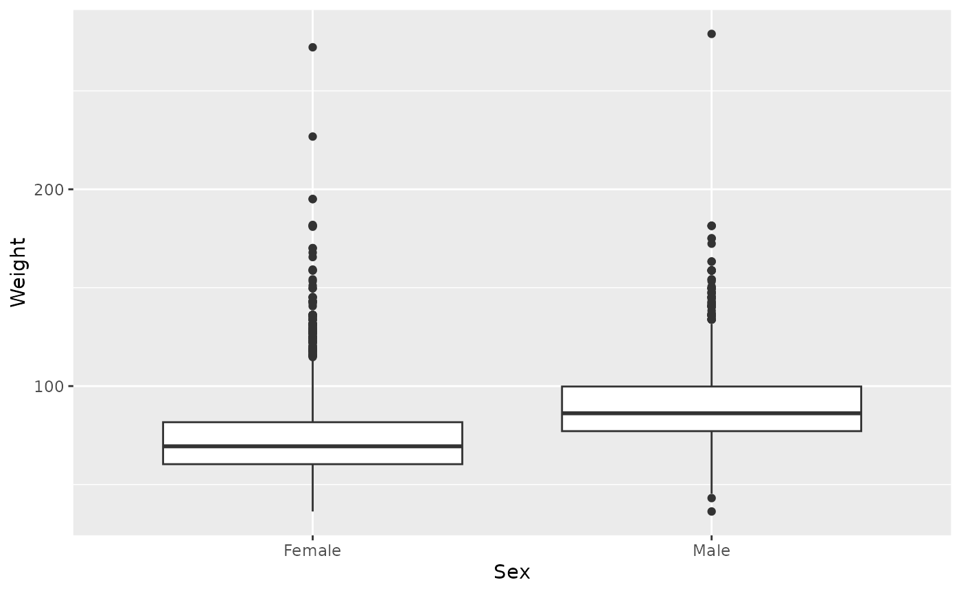

The bar in the figure is the median weight, the box represents upper and lower quartile of the data, the whiskers extend to 1.5 times the inter-quartile range. Points outside the whiskers represent potential outliers. The figure shows the difference in Female and Male weights, as well as a skew in the weight distribution of both Female and Male respondents.

Another way to view this sort of data is as a histogram…

brfss_2010 |> filter(Sex == "Male") |>
    ggplot() +
    aes(x = Weight) +
    geom_histogram(col = "white")
## `stat_bin()` using `bins = 30`. Pick better value with `binwidth`.
## Warning: Removed 49 rows containing non-finite outside the scale range
## (`stat_bin()`).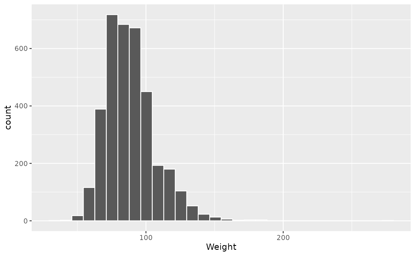

… or when comparing distributions as a density plot

ggplot(brfss_2010) +
    aes(x = Weight, color = Sex) +
    geom_density()
## Warning: Removed 395 rows containing non-finite outside the scale range
## (`stat_density()`).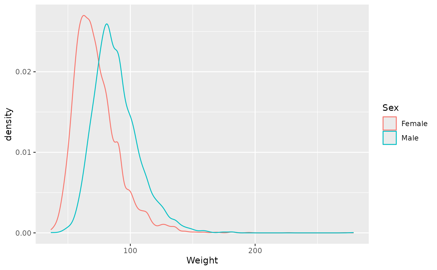

For subsequent work, note that log-transformed Weight reduces the most extreme values so the distribution is more Normal.

ggplot(brfss_2010) +
    aes(x = log10(Weight), color = Sex) +
    geom_density()
## Warning: Removed 395 rows containing non-finite outside the scale range
## (`stat_density()`).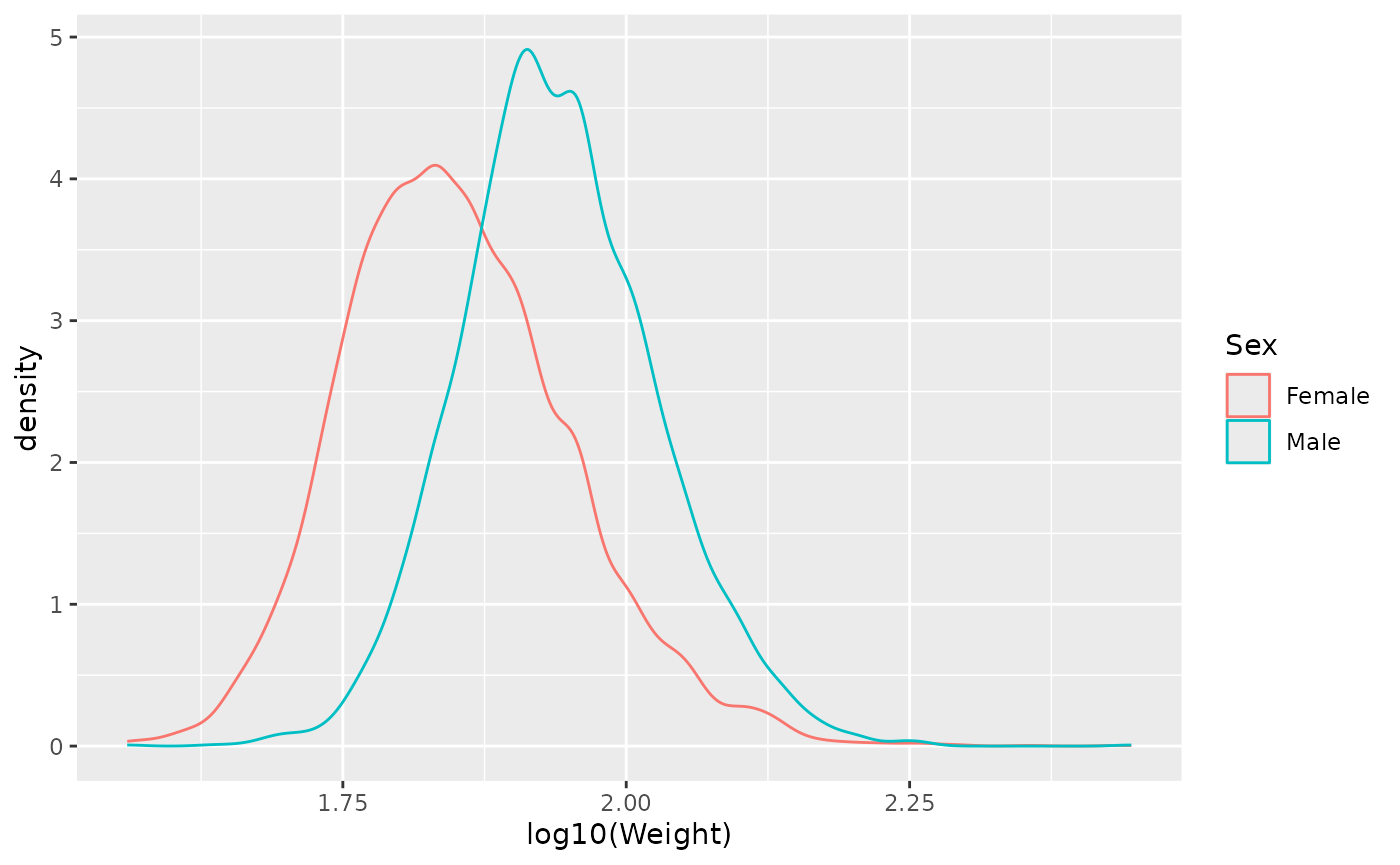

Scatter plots

Presumably taller people are heavier than shorter people. Replace ‘Sex’ with ‘Height’ in aes(), and replace geom_boxplot() with geom_point() to generate a scatter plot showing this relationship

ggplot(brfss_2010) +
    aes(x = Height, y = Weight) +
    geom_point()
## Warning: Removed 450 rows containing missing values or values outside the scale range
## (`geom_point()`).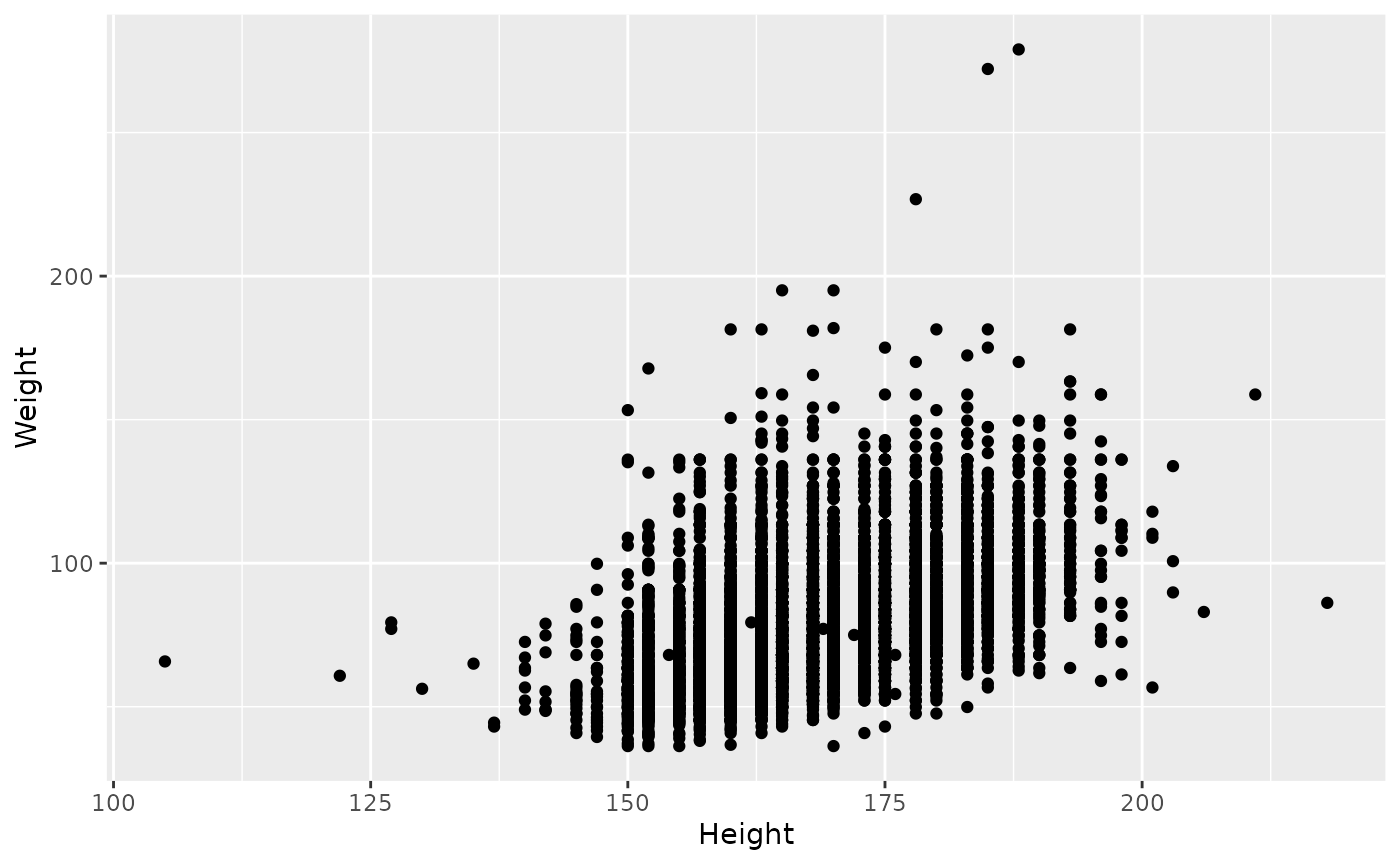

Yes there looks like a relationship. Add geom_smooth(method = "lm") to fit a smoothed relationship to the points; method = "lm" indicates that the smoothed line should be a linear regression.

ggplot(brfss_2010) +
    aes(x = Height, y = Weight) +
    geom_point() +
    geom_smooth(method = "lm")
## `geom_smooth()` using formula = 'y ~ x'
## Warning: Removed 450 rows containing non-finite outside the scale range
## (`stat_smooth()`).
## Warning: Removed 450 rows containing missing values or values outside the scale range
## (`geom_point()`).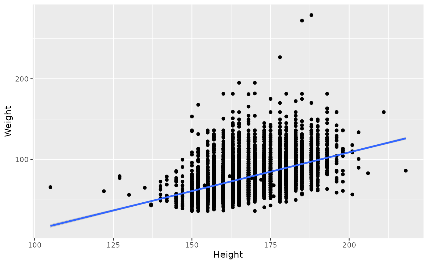

The relationship between height and weight likely depends on sex. Add color = Sex to the aes() argument, so each geom (both points and smoothed line) is colored by Sex.

ggplot(brfss_2010) +
    aes(x = Height, y = Weight, color = Sex) +
    geom_point() +
    geom_smooth(method = "lm")
## `geom_smooth()` using formula = 'y ~ x'
## Warning: Removed 450 rows containing non-finite outside the scale range
## (`stat_smooth()`).
## Warning: Removed 450 rows containing missing values or values outside the scale range
## (`geom_point()`).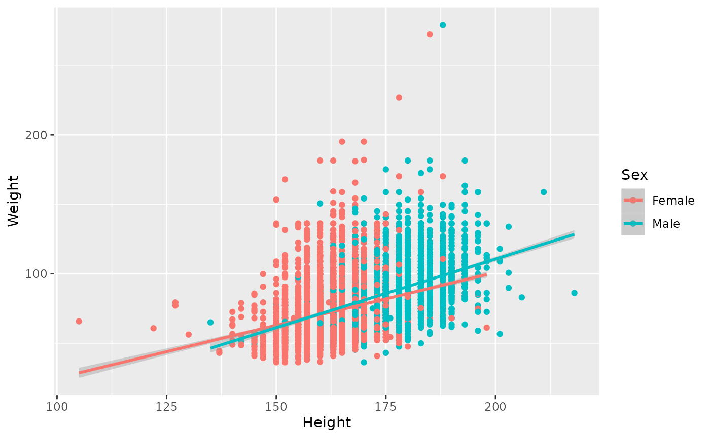

The lines cover the range of values for each sex; the relationship between height and weight appears slightly steeper for males than females.

Has the relationship between height and weight of males changed between 1990 and 2010? Change the dataset to brfss_male, color by Year, and add a title to the plot so that we know a little bit more about the relationship. Also, explore a data transformation by using the log of weight

ggplot(brfss_male) +
    aes(x = Height, y = log10(Weight), color = Year) +
    geom_point() +
    geom_smooth(method = "lm") +
    labs(title = "BRFSS Male Subset")
## `geom_smooth()` using formula = 'y ~ x'
## Warning: Removed 104 rows containing non-finite outside the scale range
## (`stat_smooth()`).
## Warning: Removed 104 rows containing missing values or values outside the scale range
## (`geom_point()`).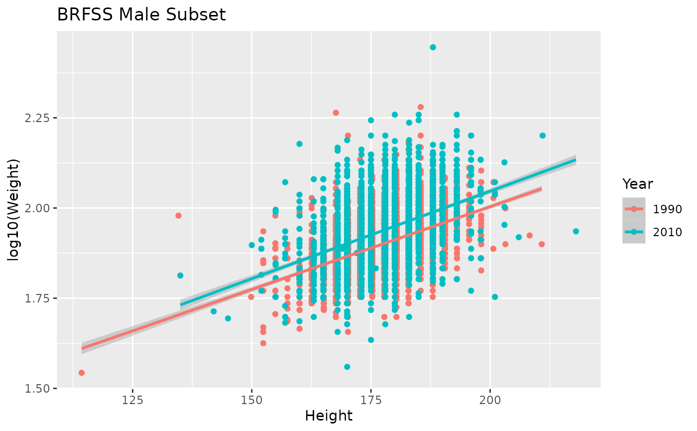

The figure suggests that 2010 males are heavier than 1990 males at all heights, and hints that the relationship between weight and height is steeper in 2010; a formal statistical analysis is required for further confidence.

Statistical analysis

This section illustrates basic statistical tests; it would be interesting to sit down with a statistician to discuss the subtleties of a more correct analysis.

We will explroe base R functions

t.test() for performing two-sample t-tests.
wilcox.test(), a non-parametric two-sample test.
lm() to fit a linear model (regression).
summary() to summarize the result of the linear model as an ANOVA table with R-squared measures summarizing goodness of fit.

Difference between groups

Here is a partial summary of the brfss_2010 data subset

brfss_2010 |>
    group_by(Sex) |>
    summarize(
        n = n(),
        ave_age = mean(Age, na.rm = TRUE),
        ave_wt = mean(Weight, na.rm = TRUE),
        ave_ht = mean(Height, na.rm = TRUE)
    )
## # A tibble: 2 × 5
##   Sex        n ave_age ave_wt ave_ht
##   <fct>  <int>   <dbl>  <dbl>  <dbl>
## 1 Female  6321    57.1   73.0   163.
## 2 Male    3679    56.2   88.8   178.

Is there statistical support for the small difference between average ages of Female and Male respondents?

Use t.test() to compare two groups. After studying the help page ?t.test, we use the ‘formula’ notation to test for differences in Age as a function of Sex, Age ~ Sex, using the subset brfss_2010 as the data source.

t.test(Age ~ Sex, brfss_2010)
## 
##  Welch Two Sample t-test
## 
## data:  Age by Sex
## t = 2.4497, df = 7768.7, p-value = 0.01432
## alternative hypothesis: true difference in means between group Female and group Male is not equal to 0
## 95 percent confidence interval:
##  0.1674909 1.5091167
## sample estimates:
## mean in group Female   mean in group Male 
##             57.08824             56.24993

The summary reports (at the bottom) mean ages of Male and Female respondents consistent with our own calculations, so we know we have not made some kind of serious blunder in formulating the test. The t-statistic of 2.4497162, with P-value 0.0143188 is significant.

What about differences in Male Weight between 1990 and 2010?

t.test(Weight ~ Year, brfss_male)
## 
##  Welch Two Sample t-test
## 
## data:  Weight by Year
## t = -20.751, df = 6549.4, p-value < 2.2e-16
## alternative hypothesis: true difference in means between group 1990 and group 2010 is not equal to 0
## 95 percent confidence interval:
##  -8.390845 -6.942327
## sample estimates:
## mean in group 1990 mean in group 2010 
##           81.17999           88.84657

Conversation with a statistician might make us concerned about whether assumptions of the t-test are fully satisfied, e.g., the data are supposed to be normally distributed, but as we saw in the box plots weights are skewed. We could try to transform the data (formal approaches to assess appropriateness of data transformations are available), e.g., by using log Weight

t.test(log10(Weight) ~ Year, brfss_male)
## 
##  Welch Two Sample t-test
## 
## data:  log10(Weight) by Year
## t = -20.202, df = 6985.4, p-value < 2.2e-16
## alternative hypothesis: true difference in means between group 1990 and group 2010 is not equal to 0
## 95 percent confidence interval:
##  -0.03971348 -0.03268805
## sample estimates:
## mean in group 1990 mean in group 2010 
##           1.903711           1.939912

Or we might use a statistic like the Wilcoxon test that makes fewer assumptions about the underlying statistical distribution.

wilcox.test(Weight ~ Year, brfss_male)
## 
##  Wilcoxon rank sum test with continuity correction
## 
## data:  Weight by Year
## W = 5754766, p-value < 2.2e-16
## alternative hypothesis: true location shift is not equal to 0

Regardless of the details of the analysis, the difference in Male Weight between 1990 and 2010 is highly significant.

Linear regression

The ‘BRFSS Male Subset’ figure shows linear relations between the square root of Weight and Height in each year.

ggplot(brfss_male) +
    aes(x = Height, y = log10(Weight), color = Year) +
    geom_point() +
    geom_smooth(method = "lm") +
    labs(title = "BRFSS Male Subset")
## `geom_smooth()` using formula = 'y ~ x'
## Warning: Removed 104 rows containing non-finite outside the scale range
## (`stat_smooth()`).
## Warning: Removed 104 rows containing missing values or values outside the scale range
## (`geom_point()`).

How would we calculate this regression, and assess its significance? We focus on Male 2010 data.

brfss_male_2010 <-
    brfss_male |>
    filter(Year == "2010")

The answer is to fit a linear regression to the data. In R, this is done by fitting a linear model (lm()) and then summarizing the result.

## fit the linear model
fit <- lm(log10(Weight) ~ Height, brfss_male_2010)

## summarize the fit, including a statistical assessment of the fit
summary(fit)
## 
## Call:
## lm(formula = log10(Weight) ~ Height, data = brfss_male_2010)
## 
## Residuals:
##      Min       1Q   Median       3Q      Max 
## -0.34142 -0.05229 -0.00645  0.04462  0.45706 
## 
## Coefficients:
##              Estimate Std. Error t value Pr(>|t|)    
## (Intercept) 1.0767107  0.0309565   34.78   <2e-16 ***
## Height      0.0048498  0.0001737   27.91   <2e-16 ***
## ---
## Signif. codes:  0 '***' 0.001 '**' 0.01 '*' 0.05 '.' 0.1 ' ' 1
## 
## Residual standard error: 0.07824 on 3617 degrees of freedom
##   (60 observations deleted due to missingness)
## Multiple R-squared:  0.1772, Adjusted R-squared:  0.177 
## F-statistic: 779.2 on 1 and 3617 DF,  p-value: < 2.2e-16

The ANOVA table shows that the relationship is highly significant. The ‘Adjusted R-squared’ value indicates that about 17% of the variation in Weight is accounted for by Height. The estimated coefficient associated with Height is the slope of the line, indicating that the square root of Weight increases by about 0.0048498 for every increase in Height of 1 cm.

As an aside, one might hope that plot(fit) would plot the regression line. Actually, it creates a series of diagnostic plots that help us assess the appropriateness of our choice of a linear model for describing this data.

More advanced analysis using R to test, e.g., for differences in the intercept or slope of the regression in 1990 versus 2010 are straight-forward to implement, but require more sophisticated statistical understanding.

Acute Lymphocytic Leukemia (ALL)

This data set is from an old microarray experiment investigating acute lymphocytic leukemia (ALL) (PMID 14684422, 16243790; the data has been extracted from the ALL Bioconductor package). We focus on phenotypes of 128 patients.

We use many of the sample dplyr functions as in the BRFSS data set, but encounter a number of new R functions useful for specific tasks.

ifelse() to compose a new vector based on values in a logical vector.
startsWith() to test whether each element of a character vector starts with a particular prefix.
%in%, used as lhs %in% rhs asks whether each element in the vector lhs is a member of the vector rhs.

Data input

Use readr::read_csv() to input the ‘ALL.csv’ file.

all_file <- file.choose() # look for 'Rpg520/week-04/extdata/all.csv'
all <- readr::read_csv(all_file)

glimpse(all)
## Rows: 128
## Columns: 21
## $ cod              <chr> "1005", "1010", "3002", "4006", "4007", "4008", "4010…
## $ diagnosis        <chr> "5/21/1997", "3/29/2000", "6/24/1998", "7/17/1997", "…
## $ sex              <chr> "M", "M", "F", "M", "M", "M", "F", "M", "M", "M", "M"…
## $ age              <dbl> 53, 19, 52, 38, 57, 17, 18, 16, 15, 40, 33, 55, 5, 18…
## $ BT               <chr> "B2", "B2", "B4", "B1", "B2", "B1", "B1", "B1", "B2",…
## $ remission        <chr> "CR", "CR", "CR", "CR", "CR", "CR", "CR", "CR", "CR",…
## $ CR               <chr> "CR", "CR", "CR", "CR", "CR", "CR", "CR", "CR", "CR",…
## $ date.cr          <chr> "8/6/1997", "6/27/2000", "8/17/1998", "9/8/1997", "9/…
## $ `t(4;11)`        <lgl> FALSE, FALSE, NA, TRUE, FALSE, FALSE, FALSE, FALSE, F…
## $ `t(9;22)`        <lgl> TRUE, FALSE, NA, FALSE, FALSE, FALSE, FALSE, FALSE, F…
## $ cyto.normal      <lgl> FALSE, FALSE, NA, FALSE, FALSE, FALSE, FALSE, FALSE, …
## $ citog            <chr> "t(9;22)", "simple alt.", NA, "t(4;11)", "del(6q)", "…
## $ mol.biol         <chr> "BCR/ABL", "NEG", "BCR/ABL", "ALL1/AF4", "NEG", "NEG"…
## $ `fusion protein` <chr> "p210", NA, "p190", NA, NA, NA, NA, NA, NA, "p190", "…
## $ mdr              <chr> "NEG", "POS", "NEG", "NEG", "NEG", "NEG", "POS", "NEG…
## $ kinet            <chr> "dyploid", "dyploid", "dyploid", "dyploid", "dyploid"…
## $ ccr              <lgl> FALSE, FALSE, FALSE, FALSE, FALSE, FALSE, FALSE, FALS…
## $ relapse          <lgl> FALSE, TRUE, TRUE, TRUE, TRUE, TRUE, TRUE, TRUE, TRUE…
## $ transplant       <lgl> TRUE, FALSE, FALSE, FALSE, FALSE, FALSE, FALSE, FALSE…
## $ f.u              <chr> "BMT / DEATH IN CR", "REL", "REL", "REL", "REL", "REL…
## $ `date last seen` <chr> NA, "8/28/2000", "10/15/1999", "1/23/1998", "11/4/199…

Exploration & cleaning

For simplicity we focus on the following columns:

‘cod’ is a unique identifier
‘sex’. We will recode this to a factor with levels ‘Female’ and ‘Male’, so that there is no ambiguity about its meaning.
‘age’.
‘BT’ represents B- or T- cell status. It is too fine-grained, so we will recode this to a new variable ‘BorT’.
‘mol.biol’ summarizes status with respect to chromosomal status. We will filter the data to contain only patients with values ‘BCR/ABL’ (the classic BCR / ABL inversion) or ‘NEG’ (no chromosomal changes). We will recode the result as a factor with levels ‘BCR/ABL’ and ‘NEG’.

`select()`

Use select() to select just the columns of interest. Re-assign the result to all.

all <-
    all |>
    select(cod, sex, age, BT, mol.biol)

`ifelse()` and `factor()`

‘sex’ is currently a character vector with two values ‘F’ and ‘M’, as well as missing values

all |>
    count(sex)
## # A tibble: 3 × 2
##   sex       n
##   <chr> <int>
## 1 F        42
## 2 M        83
## 3 NA        3

We can remove individuals whose sex is unknown using filter(!is.na(sex)). Use ifelse() to translate ‘F’ and ‘M’ to ‘Female’ and ‘Male’, and then factor() so that this column is a factor

all  |>
    filter(!is.na(sex)) |>
    mutate(
        sex = factor(
            ifelse(sex == "F", "Female", "Male"),
            levels = c("Female", "Male")
        )
    )
## # A tibble: 125 × 5
##    cod   sex      age BT    mol.biol
##    <chr> <fct>  <dbl> <chr> <chr>   
##  1 1005  Male      53 B2    BCR/ABL 
##  2 1010  Male      19 B2    NEG     
##  3 3002  Female    52 B4    BCR/ABL 
##  4 4006  Male      38 B1    ALL1/AF4
##  5 4007  Male      57 B2    NEG     
##  6 4008  Male      17 B1    NEG     
##  7 4010  Female    18 B1    NEG     
##  8 4016  Male      16 B1    NEG     
##  9 6002  Male      15 B2    NEG     
## 10 8001  Male      40 B2    BCR/ABL 
## # ℹ 115 more rows

`startsWith()`

The BT column describes whether individuals have B- or T-cell ALL. There are several different grades of each.

all |>
    count(BT)
## # A tibble: 10 × 2
##    BT        n
##    <chr> <int>
##  1 B         5
##  2 B1       19
##  3 B2       36
##  4 B3       23
##  5 B4       12
##  6 T         5
##  7 T1        1
##  8 T2       15
##  9 T3       10
## 10 T4        2

We are interested in simplifying this to just two values, ‘B’ or ‘T’, based on the first letter of each vector element. The startsWith() function returns TRUE each time an element of the first argument starts with the second argument.

x <- c("B", "B1", "T")
startsWith(x, "B")
## [1]  TRUE  TRUE FALSE

We can combine this with ifelse() and factor() to mutate BT

all |>
    mutate(
        BT = factor(
            ifelse(startsWith(BT, "B"), "B", "T"),
            levels = c("B", "T")
        )
    )
## # A tibble: 128 × 5
##    cod   sex     age BT    mol.biol
##    <chr> <chr> <dbl> <fct> <chr>   
##  1 1005  M        53 B     BCR/ABL 
##  2 1010  M        19 B     NEG     
##  3 3002  F        52 B     BCR/ABL 
##  4 4006  M        38 B     ALL1/AF4
##  5 4007  M        57 B     NEG     
##  6 4008  M        17 B     NEG     
##  7 4010  F        18 B     NEG     
##  8 4016  M        16 B     NEG     
##  9 6002  M        15 B     NEG     
## 10 8001  M        40 B     BCR/ABL 
## # ℹ 118 more rows

`%in%`

‘mol.biol’ is also a character vector with several different values.

all |>
    count(mol.biol)
## # A tibble: 6 × 2
##   mol.biol     n
##   <chr>    <int>
## 1 ALL1/AF4    10
## 2 BCR/ABL     37
## 3 E2A/PBX1     5
## 4 NEG         74
## 5 NUP-98       1
## 6 p15/p16      1

We will filter all to only include ‘BCR/ABL’ or ‘NEG’ samples using %in%. %in% is an ‘infix’ operator (like ~) with a left-hand side and a right-hand side. The left-hand side is a vector of values that we are interested in. The right-hand side is also a vector, and represents a (mathematical) ‘set’ of values. %in% asks, for each element of the left-hand size, if the element is a member of the set on the right hand side.

x <- c(1, 2, 3, 4, 5)
x %in% c(2, 5)
## [1] FALSE  TRUE FALSE FALSE  TRUE

Filtering the all dataset is accomplished with

all |>
    filter(mol.biol %in% c("BCR/ABL", "NEG"))
## # A tibble: 111 × 5
##    cod   sex     age BT    mol.biol
##    <chr> <chr> <dbl> <chr> <chr>   
##  1 1005  M        53 B2    BCR/ABL 
##  2 1010  M        19 B2    NEG     
##  3 3002  F        52 B4    BCR/ABL 
##  4 4007  M        57 B2    NEG     
##  5 4008  M        17 B1    NEG     
##  6 4010  F        18 B1    NEG     
##  7 4016  M        16 B1    NEG     
##  8 6002  M        15 B2    NEG     
##  9 8001  M        40 B2    BCR/ABL 
## 10 8011  M        33 B3    BCR/ABL 
## # ℹ 101 more rows

Re-coding the filtered values of ‘mol.biol’ uses factor() in a way that we have already seen with ‘sex’.

Data cleaning pipeline

Putting these filtering and re-coding steps together, our initial cleaning results in

all_subset <-
    all |>
    ## columns of interest
    select(cod, sex, age, BT, mol.biol) |>
    ## rows of interest
    filter(
        !is.na(sex),
        mol.biol %in% c("BCR/ABL", "NEG")
    ) |>
    ## re-coding sex, mol.bio, BT
    mutate(
        sex = factor(
            ifelse(sex == "F", "Female", "Male"),
            levels = c("Female", "Male")
        ),
        BT = factor(
            ifelse(startsWith(BT, "B"), "B", "T"),
            levels = c("B", "T")
        ),
        mol.biol = factor(mol.biol, levels = c("BCR/ABL", "NEG"))
    )

Data exploration

A basic characterize of our subset might group by sex and summarize the number and average age of each group.

all_subset |>
    group_by(sex) |>
    summarize(
        n = n(),
        av_age = mean(age, na.rm = TRUE)
    )
## # A tibble: 2 × 3
##   sex        n av_age
##   <fct>  <int>  <dbl>
## 1 Female    35   34.8
## 2 Male      74   30.9

There are about twice as many Male as Female samples; the average age of Female samples is about 4 years older than Male samples.

We can visualize the distribution of ages in several ways, as illustrated in the previous case study. Here we create a box plot with geom_boxplot(), then overlay the individual points using geom_jitter() (this geom displays each point but with a bit of ‘jitter’ away from its actual value – instead of being plotted exactly on the ‘Female’ or ‘Male’ line, the points are offset a random amount).

ggplot(all_subset) +
    aes(x = sex, y = age) +
    geom_boxplot() +
    geom_jitter(width = .2)
## Warning: Removed 2 rows containing non-finite outside the scale range
## (`stat_boxplot()`).
## Warning: Removed 2 rows containing missing values or values outside the scale range
## (`geom_point()`).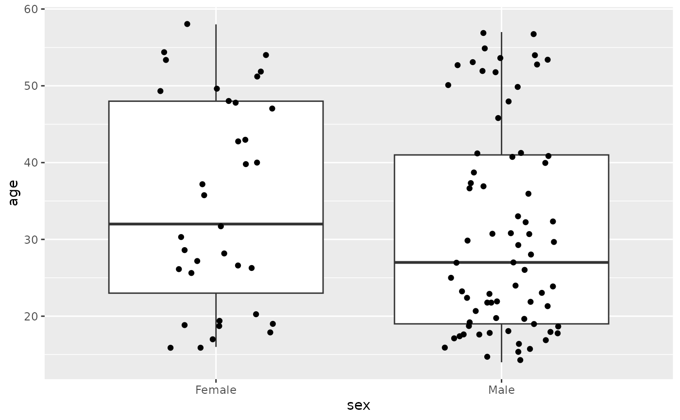

The following table counts the number of ‘BCR/ABL’ and ‘NEG’ among ‘Female’ and ‘Male’ samples; it seems like there is a disproportionate number of ‘Male’ ‘NEG’ (chromosomally normal) individuals.

all_subset |>
    count(mol.biol, sex) |>
    tidyr::pivot_wider(names_from = "sex", values_from = "n")
## # A tibble: 2 × 3
##   mol.biol Female  Male
##   <fct>     <int> <int>
## 1 BCR/ABL      16    21
## 2 NEG          19    53

Here is a similar tally of B- and T-cell ALL for ‘Female’ and ‘Male’ samples

all_subset |>
    count(BT, sex) |>
    tidyr::pivot_wider(names_from = "sex", values_from = "n")
## # A tibble: 2 × 3
##   BT    Female  Male
##   <fct>  <int> <int>
## 1 B         28    50
## 2 T          7    24

… and a count of ‘BT’ and ‘mol.biol’ by sex

all_subset |>
    count(BT, mol.biol, sex) |>
    tidyr::pivot_wider(names_from = "sex", values_from = "n")
## # A tibble: 3 × 4
##   BT    mol.biol Female  Male
##   <fct> <fct>     <int> <int>
## 1 B     BCR/ABL      16    21
## 2 B     NEG          12    29
## 3 T     NEG           7    24

Note that there are not T-cell, BCR/ABL samples. Is this for biological reasons, or is an artifact of the procedures used in data collection? Does it limit or bias the statistical questions that can be asked?

Statistical analysis

A t-test indicates that the difference in Male and Female age noted above is not statistically significant

t.test(age ~ sex, all_subset)
## 
##  Welch Two Sample t-test
## 
## data:  age by sex
## t = 1.3901, df = 66.316, p-value = 0.1691
## alternative hypothesis: true difference in means between group Female and group Male is not equal to 0
## 95 percent confidence interval:
##  -1.687236  9.424537
## sample estimates:
## mean in group Female   mean in group Male 
##             34.77143             30.90278

We noted differences in the number ‘BCR/ABL’ and ‘NEG’ samples with respect to sex. A Chi-squared test can be used to assess whether these differences are statistically significant. Look at the help page ?chisq.test. The idea is that the first argument is a vector of observations of one variable (e.g., mol.biol) and the second argument is the second variable (sex). Unlike t.test, there is no data= argument, and no formula (~) interface. In base R one might use $ to access individual columns of a tibble, so the test could be performed with

chisq.test(all_subset$mol.biol, all_subset$sex)

A convenient variation of this is to use the function with(), which allows one to write the test as

all_subset |>
    with(chisq.test(mol.biol, sex))
## 
##  Pearson's Chi-squared test with Yates' continuity correction
## 
## data:  mol.biol and sex
## X-squared = 2.4586, df = 1, p-value = 0.1169

The P-value indicates that the differences in counts of ‘BCR/ABL’ and ‘NEG’ observed between ‘Female’ and ‘Male’ are not statistically supported. A similar conclusion applies with BT and sex.

all_subset |>
    with(chisq.test(BT, sex))
## 
##  Pearson's Chi-squared test with Yates' continuity correction
## 
## data:  BT and sex
## X-squared = 1.2454, df = 1, p-value = 0.2644

Session information

For reproducibility, I record the software versions used to create this document

sessionInfo()
## R version 4.3.3 (2024-02-29)
## Platform: x86_64-pc-linux-gnu (64-bit)
## Running under: Ubuntu 22.04.4 LTS
## 
## Matrix products: default
## BLAS:   /usr/lib/x86_64-linux-gnu/openblas-pthread/libblas.so.3 
## LAPACK: /usr/lib/x86_64-linux-gnu/openblas-pthread/libopenblasp-r0.3.20.so;  LAPACK version 3.10.0
## 
## locale:
##  [1] LC_CTYPE=C.UTF-8       LC_NUMERIC=C           LC_TIME=C.UTF-8       
##  [4] LC_COLLATE=C.UTF-8     LC_MONETARY=C.UTF-8    LC_MESSAGES=C.UTF-8   
##  [7] LC_PAPER=C.UTF-8       LC_NAME=C              LC_ADDRESS=C          
## [10] LC_TELEPHONE=C         LC_MEASUREMENT=C.UTF-8 LC_IDENTIFICATION=C   
## 
## time zone: UTC
## tzcode source: system (glibc)
## 
## attached base packages:
## [1] stats     graphics  grDevices utils     datasets  methods   base     
## 
## other attached packages:
## [1] ggplot2_3.5.0 dplyr_1.1.4  
## 
## loaded via a namespace (and not attached):
##  [1] sass_0.4.8        utf8_1.2.4        generics_0.1.3    tidyr_1.3.1      
##  [5] lattice_0.22-5    stringi_1.8.3     hms_1.1.3         digest_0.6.34    
##  [9] magrittr_2.0.3    evaluate_0.23     grid_4.3.3        fastmap_1.1.1    
## [13] Matrix_1.6-5      jsonlite_1.8.8    mgcv_1.9-1        purrr_1.0.2      
## [17] fansi_1.0.6       scales_1.3.0      textshaping_0.3.7 jquerylib_0.1.4  
## [21] cli_3.6.2         rlang_1.1.3       crayon_1.5.2      splines_4.3.3    
## [25] bit64_4.0.5       munsell_0.5.0     withr_3.0.0       cachem_1.0.8     
## [29] yaml_2.3.8        tools_4.3.3       parallel_4.3.3    tzdb_0.4.0       
## [33] memoise_2.0.1     colorspace_2.1-0  vctrs_0.6.5       R6_2.5.1         
## [37] lifecycle_1.0.4   stringr_1.5.1     fs_1.6.3          bit_4.0.5        
## [41] vroom_1.6.5       ragg_1.2.7        pkgconfig_2.0.3   desc_1.4.3       
## [45] pkgdown_2.0.7     pillar_1.9.0      bslib_0.6.1       gtable_0.3.4     
## [49] glue_1.7.0        systemfonts_1.0.5 highr_0.10        xfun_0.42        
## [53] tibble_3.2.1      tidyselect_1.2.0  knitr_1.45        farver_2.1.1     
## [57] nlme_3.1-164      htmltools_0.5.7   labeling_0.4.3    rmarkdown_2.25   
## [61] readr_2.1.5       compiler_4.3.3

Introduction

US CDC Behavioral Risk Factor Surveillance System survey data

Data input

Initial cleaning

Mutate

Data exploration

Count

Summarize

Group

Filter

Visual exploration

Aesthetics & geometries: box plot, histogram, density plot

Scatter plots

Statistical analysis

Difference between groups

Linear regression

Acute Lymphocytic Leukemia (ALL)

Data input

Exploration & cleaning

select()

ifelse() and factor()

startsWith()

%in%

Data cleaning pipeline

Data exploration

Statistical analysis

Session information

`select()`

`ifelse()` and `factor()`

`startsWith()`

`%in%`