1. Accessing Human Cell Atlas Data
Martin Morgan1, Maya McDaniel, Yubo Cheng2.
Source:vignettes/A_HCA.Rmd
A_HCA.RmdOverview
R / Bioconductor packages used
The focus is on the hca package. This package emphasize dplyr and ‘tidy’ approaches to working with data.frames. Files downloaded from the HCA or CellXGene web sites can be imported into R / Bioconductor as SingleCellExperiment objects through the LoomExperiment and zellkonverter packages.
Workshop
Single-cell analysis in Bioconductor
Extensive support for single-cell analysis in Bioconductor
-
E.g., 213 packages tagged ‘SingleCell’ in the release branch
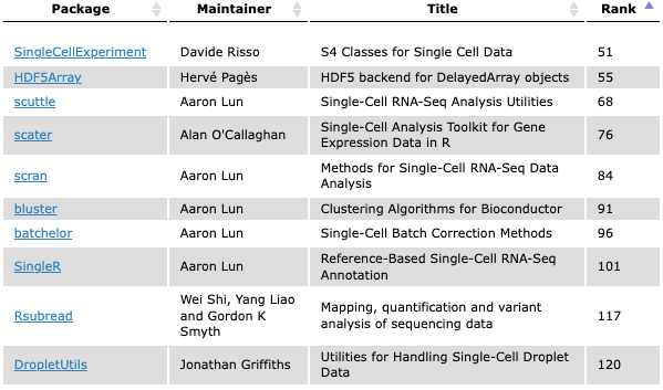
Quality control, normalization, variance modeling, data integration / batch correction, dimensionality reduction, clustering, differential expression, cell type classification, etc
Infrastructure to support large out-of-memory data, etc.
Typically, processing after a ‘count matrix’ has been obtained
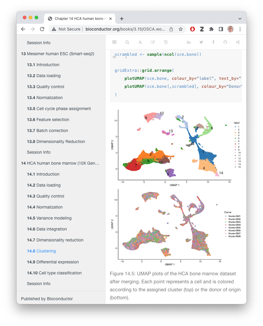
Orchestrating Single-Cell Analysis with Bioconductor (OSCA) – an amazing resource!
A quick dplyr ‘tidy’ refresher
Recall
- A
tibble()is adata.frame()but with a nicer display. - A few common commands allow many standard manipulations
-
filter(): filter to include only specific rows -
select(): select columns -
mutate(): change or add columns -
glimpes(): get a quick summary of the first rows of thetibble -
left_join(x, y, by =)is a somehat more advanced function, merging all rows of tibblexwith rows inythat match for columns specified byby=.
-
-
R introduced the ‘pipe’
|>, typically used to take the output of one command and ‘pipe’ it to the first input argument of the next command
suppressPackageStartupMessages({
    library(dplyr)
})

tbl <- as_tibble(mtcars, rownames = "car")
tbl
#> # A tibble: 32 × 12
#>    car           mpg   cyl  disp    hp  drat    wt  qsec    vs    am  gear  carb
#>    <chr>       <dbl> <dbl> <dbl> <dbl> <dbl> <dbl> <dbl> <dbl> <dbl> <dbl> <dbl>
#>  1 Mazda RX4    21       6  160    110  3.9   2.62  16.5     0     1     4     4
#>  2 Mazda RX4 …  21       6  160    110  3.9   2.88  17.0     0     1     4     4
#>  3 Datsun 710   22.8     4  108     93  3.85  2.32  18.6     1     1     4     1
#>  4 Hornet 4 D…  21.4     6  258    110  3.08  3.22  19.4     1     0     3     1
#>  5 Hornet Spo…  18.7     8  360    175  3.15  3.44  17.0     0     0     3     2
#>  6 Valiant      18.1     6  225    105  2.76  3.46  20.2     1     0     3     1
#>  7 Duster 360   14.3     8  360    245  3.21  3.57  15.8     0     0     3     4
#>  8 Merc 240D    24.4     4  147.    62  3.69  3.19  20       1     0     4     2
#>  9 Merc 230     22.8     4  141.    95  3.92  3.15  22.9     1     0     4     2
#> 10 Merc 280     19.2     6  168.   123  3.92  3.44  18.3     1     0     4     4
#> # … with 22 more rows
#> # ℹ Use `print(n = ...)` to see more rows
tbl |>
    filter(cyl == 6) |>
    select(car, mpg, disp, hp) |>
    mutate(`L/100km` = 235.2 / mpg) # Liters per 100 km
#> # A tibble: 7 × 5
#>   car              mpg  disp    hp `L/100km`
#>   <chr>          <dbl> <dbl> <dbl>     <dbl>
#> 1 Mazda RX4       21    160    110      11.2
#> 2 Mazda RX4 Wag   21    160    110      11.2
#> 3 Hornet 4 Drive  21.4  258    110      11.0
#> 4 Valiant         18.1  225    105      13.0
#> 5 Merc 280        19.2  168.   123      12.2
#> 6 Merc 280C       17.8  168.   123      13.2
#> 7 Ferrari Dino    19.7  145    175      11.9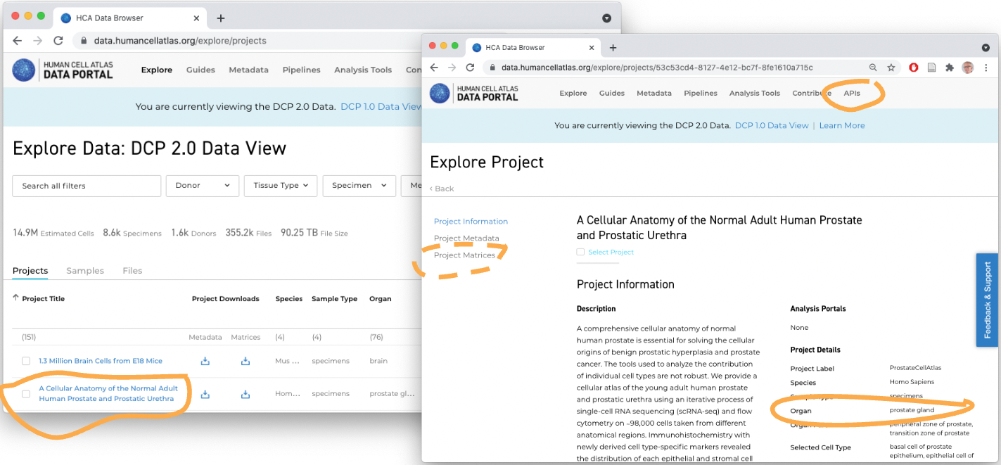
Working with HCA data
Why use an R script when the Data Portal exists?
- Easily reproducible
- Flexible exploration of rich & complex data
- Direct integration with Bioconductor single-cell workflows
Load required packages
suppressPackageStartupMessages({
    library(hca)
    library(LoomExperiment)
    library(SingleCellExperiment)
})
Discover projects
## basic information, like HCA data portal
p <- projects()
p
#> # A tibble: 267 × 14
#> projectId proje…¹ genus…² sampl…³ speci…⁴ speci…⁵ selec…⁶ libra…⁷ nucle…⁸
#> <chr> <chr> <list> <list> <list> <list> <list> <list> <list>
#> 1 74b6d569-3b1… 1.3 Mi… <chr> <chr> <chr> <chr> <chr> <chr> <chr>
#> 2 53c53cd4-812… A Cell… <chr> <chr> <chr> <chr> <chr> <chr> <chr>
#> 3 7027adc6-c9c… A Cell… <chr> <chr> <chr> <chr> <chr> <chr> <chr>
#> 4 94e4ee09-9b4… A Huma… <chr> <chr> <chr> <chr> <chr> <chr> <chr>
#> 5 60ea42e1-af4… A Prot… <chr> <chr> <chr> <chr> <chr> <chr> <chr>
#> 6 ef1e3497-515… A Sing… <chr> <chr> <chr> <chr> <chr> <chr> <chr>
#> 7 f86f1ab4-1fb… A Sing… <chr> <chr> <chr> <chr> <chr> <chr> <chr>
#> 8 602628d7-c03… A Sing… <chr> <chr> <chr> <chr> <chr> <chr> <chr>
#> 9 c1810dbc-16d… A cell… <chr> <chr> <chr> <chr> <chr> <chr> <chr>
#> 10 c0518445-3b3… A cell… <chr> <chr> <chr> <chr> <chr> <chr> <chr>
#> # … with 257 more rows, 5 more variables: pairedEnd <list>, workflow <list>,
#> # specimenDisease <list>, donorDisease <list>, developmentStage <list>, and
#> # abbreviated variable names ¹projectTitle, ²genusSpecies, ³sampleEntityType,
#> # ⁴specimenOrgan, ⁵specimenOrganPart, ⁶selectedCellType,
#> # ⁷libraryConstructionApproach, ⁸nucleicAcidSource
#> # ℹ Use `print(n = ...)` to see more rows, and `colnames()` to see all variable namesColumns with type <list> usually have some
projects with 0, 1, 2, or more of the corresponding column. This is more
clearly displayed when the dplyr print method allocates more room per
column, or when using glimpse(), or by pulling the column
from the table.
p |>
    select(specimenOrganPart)
#> # A tibble: 267 × 1
#>    specimenOrganPart
#>    <list>
#>  1 <chr [1]>
#>  2 <chr [2]>
#>  3 <chr [0]>
#>  4 <chr [0]>
#>  5 <chr [1]>
#>  6 <chr [4]>
#>  7 <chr [0]>
#>  8 <chr [3]>
#>  9 <chr [0]>
#> 10 <chr [6]>
#> # … with 257 more rows
#> # ℹ Use `print(n = ...)` to see more rows
p |>
    glimpse()
#> Rows: 267
#> Columns: 14
#> $ projectId                   <chr> "74b6d569-3b11-42ef-b6b1-a0454522b4a0", "5…
#> $ projectTitle                <chr> "1.3 Million Brain Cells from E18 Mice", "…
#> $ genusSpecies                <list> "Mus musculus", "Homo sapiens", "Mus musc…
#> $ sampleEntityType            <list> "specimens", "specimens", "specimens", <"…
#> $ specimenOrgan               <list> "brain", "prostate gland", "heart", "live…
#> $ specimenOrganPart           <list> "cortex", <"peripheral zone of prostate",…
#> $ selectedCellType            <list> "neuron", <"basal cell of prostate epithe…
#> $ libraryConstructionApproach <list> "10x 3' v2", "10X v2 sequencing", "10X 3'…
#> $ nucleicAcidSource           <list> "single cell", "single cell", "single cel…
#> $ pairedEnd                   <list> FALSE, FALSE, FALSE, FALSE, TRUE, FALSE, …
#> $ workflow                    <list> <>, <"optimus_post_processing_v1.0.0", "o…
#> $ specimenDisease             <list> "normal", "normal", "normal", <"hepatocel…
#> $ donorDisease                <list> "normal", "normal", "normal", <"cholangio…
#> $ developmentStage            <list> "mouse embryo stage", "human adult stage"…
p |>
    head() |>
    pull(specimenOrganPart)
#> [[1]]
#> [1] "cortex"
#>
#> [[2]]
#> [1] "peripheral zone of prostate" "transition zone of prostate"
#>
#> [[3]]
#> character(0)
#>
#> [[4]]
#> character(0)
#>
#> [[5]]
#> [1] "saliva"
#>
#> [[6]]
#> [1] "epithelium of bronchus"       "epithelium of trachea"
#> [3] "inferior nasal concha"        "terminal bronchus epithelium"
Using hca_view(p) displays the data in a graphical
widget that allows selection of one or several projects.
The table can be expanded so that there is one row for each
specimenOrganPart, rather than for each project; it is
usually not productive to unnest multiple columns, because this leads to
a combinatorial number of rows.
p |>
tidyr::unnest(specimenOrganPart)
#> # A tibble: 424 × 14
#> projectId proje…¹ genus…² sampl…³ speci…⁴ speci…⁵ selec…⁶ libra…⁷ nucle…⁸
#> <chr> <chr> <list> <list> <list> <chr> <list> <list> <list>
#> 1 74b6d569-3b1… 1.3 Mi… <chr> <chr> <chr> cortex <chr> <chr> <chr>
#> 2 53c53cd4-812… A Cell… <chr> <chr> <chr> periph… <chr> <chr> <chr>
#> 3 53c53cd4-812… A Cell… <chr> <chr> <chr> transi… <chr> <chr> <chr>
#> 4 60ea42e1-af4… A Prot… <chr> <chr> <chr> saliva <chr> <chr> <chr>
#> 5 ef1e3497-515… A Sing… <chr> <chr> <chr> epithe… <chr> <chr> <chr>
#> 6 ef1e3497-515… A Sing… <chr> <chr> <chr> epithe… <chr> <chr> <chr>
#> 7 ef1e3497-515… A Sing… <chr> <chr> <chr> inferi… <chr> <chr> <chr>
#> 8 ef1e3497-515… A Sing… <chr> <chr> <chr> termin… <chr> <chr> <chr>
#> 9 602628d7-c03… A Sing… <chr> <chr> <chr> annulu… <chr> <chr> <chr>
#> 10 602628d7-c03… A Sing… <chr> <chr> <chr> nucleu… <chr> <chr> <chr>
#> # … with 414 more rows, 5 more variables: pairedEnd <list>, workflow <list>,
#> # specimenDisease <list>, donorDisease <list>, developmentStage <list>, and
#> # abbreviated variable names ¹projectTitle, ²genusSpecies, ³sampleEntityType,
#> # ⁴specimenOrgan, ⁵specimenOrganPart, ⁶selectedCellType,
#> # ⁷libraryConstructionApproach, ⁸nucleicAcidSource
#> # ℹ Use `print(n = ...)` to see more rows, and `colnames()` to see all variable namesArguments to projects() allow information to be returned
in different formats, or to return much more information about each
project. Using as = "list" produces a nested data structure
with all information provided by the HCA Data Portal; exploring this
data is facilitated by listveiwer::jsonedit(), using
as = "lol" and lol_* functions in the hca package, or perhaps
cellxgenedp::jmespath().
## all information, as a list-of-lists
pl <- projects(as = "list")
lengths(pl)
#> pagination termFacets       hits
#>          8         36        267
An alternative to working with all projects is to apply filters during the original query. For instance, to select subsets of projects, e.g., studying liver. It is possible to specify several filters at once, as we will see below.
liver_filter <- filters(
    specimenOrgan = list(is = "liver")
)
liver_projects <- projects(liver_filter)
liver_projects |>
    select(projectId, projectTitle)
#> # A tibble: 23 × 2
#>    projectId                            projectTitle
#>    <chr>                                <chr>
#>  1 94e4ee09-9b4b-410a-84dc-a751ad36d0df A Human Liver Cell Atlas reveals Hetero…
#>  2 a9301beb-e9fa-42fe-b75c-84e8a460c733 A human cell atlas of fetal gene expres…
#>  3 c31fa434-c9ed-4263-a9b6-d9ffb9d44005 A single-cell atlas of chromatin access…
#>  4 8ab8726d-81b9-4bd2-acc2-4d50bee786b4 An organoid and multi-organ development…
#>  5 04ad400c-58cb-40a5-bc2b-2279e13a910b Blood and immune development in human f…
#>  6 c7c54245-548b-4d4f-b15e-0d7e238ae6c8 Construction of a single-cell transcrip…
#>  7 a9f5323a-ce71-471c-9caf-04cc118fd1d7 Decoding Human Megakaryocyte Development
#>  8 f2fe82f0-4454-4d84-b416-a885f3121e59 Decoding human fetal liver haematopoies…
#>  9 ccef38d7-aa92-4010-9621-c4c7b1182647 Dissecting the clonal nature of allelic…
#> 10 4d6f6c96-2a83-43d8-8fe1-0f53bffd4674 Dissecting the human liver cellular lan…
#> # … with 13 more rows
#> # ℹ Use `print(n = ...)` to see more rows

## facet options available for filtering: facet_options()
Main functions for exploring HCA data
-
projects(): finding projects of interest. -
bundles(),samples(): can be useful when exploring a single project in detail. -
files(): use to download files (e.g., fastq files to start an analysis from scratch; ‘.loom’ files containing gene x cell count matrices produced by standard HCA pipelines). -
hca_next(),hca_prev()to ‘page’ through large datasets.
Discovering and downloading ‘.loom’ files
HCA standard processing pipelines
Projects with .loom files produced by the standard pipeline satisfy the following filter
standard_loom_file_filter <- filters(
    fileSource = list(is = "DCP/2 Analysis"),
    fileFormat = list(is = "loom"),
    workflow = list(is = "optimus_post_processing_v1.0.0")
)
loom_files <- files(standard_loom_file_filter)
Which projects studying the liver have a standard loom file available?
## inner_join -- projectId & projectTitles in both tibbles
liver_loom_projects <- inner_join(
liver_projects, loom_files,
by = c("projectId", "projectTitle")
)
liver_loom_projects |>
select(projectId, fileId, projectTitle, fileSize = size)
#> # A tibble: 11 × 4
#> projectId fileId proje…¹ fileS…²
#> <chr> <chr> <chr> <dbl>
#> 1 f2fe82f0-4454-4d84-b416-a885f3121e59 815e27f4-56f9-538a-a770… Decodi… 2.45e8
#> 2 f2fe82f0-4454-4d84-b416-a885f3121e59 e9ac4222-8586-5d9b-8c6d… Decodi… 5.39e9
#> 3 f2fe82f0-4454-4d84-b416-a885f3121e59 c15acbfd-268a-571c-ab78… Decodi… 1.09e9
#> 4 f2fe82f0-4454-4d84-b416-a885f3121e59 84e656b7-3740-5fa9-8f81… Decodi… 1.82e9
#> 5 4d6f6c96-2a83-43d8-8fe1-0f53bffd4674 b1f60da2-db89-556b-b89f… Dissec… 1.18e9
#> 6 c41dffbf-ad83-447c-a0e1-13e689d9b258 11f8ba42-a556-5757-a0f4… Resolv… 1.30e8
#> 7 c41dffbf-ad83-447c-a0e1-13e689d9b258 ec8fcbf6-8556-5820-af81… Resolv… 2.90e8
#> 8 c41dffbf-ad83-447c-a0e1-13e689d9b258 58ff8ba0-280d-51b3-923b… Resolv… 1.25e9
#> 9 559bb888-7829-41f2-ace5-2c05c7eb81e9 6e061337-810d-5089-a923… Single… 5.11e8
#> 10 559bb888-7829-41f2-ace5-2c05c7eb81e9 8fbd3d96-dcdf-5c58-b9b5… Single… 2.96e8
#> 11 559bb888-7829-41f2-ace5-2c05c7eb81e9 0264fd26-4f63-5a35-a524… Single… 6.29e8
#> # … with abbreviated variable names ¹projectTitle, ²fileSizeChoose one project more-or-less arbitrarily, for demonstration purposes
liver_loom_projects |>
    filter(projectId == "4d6f6c96-2a83-43d8-8fe1-0f53bffd4674") |>
    glimpse()
#> Rows: 1
#> Columns: 20
#> $ projectId                   <chr> "4d6f6c96-2a83-43d8-8fe1-0f53bffd4674"
#> $ projectTitle                <chr> "Dissecting the human liver cellular lands…
#> $ genusSpecies                <list> "Homo sapiens"
#> $ sampleEntityType            <list> "specimens"
#> $ specimenOrgan               <list> "liver"
#> $ specimenOrganPart           <list> "caudate lobe"
#> $ selectedCellType            <list> <>
#> $ libraryConstructionApproach <list> "10x 3' v2"
#> $ nucleicAcidSource           <list> "single cell"
#> $ pairedEnd                   <list> FALSE
#> $ workflow                    <list> <"optimus_post_processing_v1.0.0", "optimu…
#> $ specimenDisease             <list> "normal"
#> $ donorDisease                <list> "normal"
#> $ developmentStage            <list> "human adult stage"
#> $ fileId                      <chr> "b1f60da2-db89-556b-b89f-6fbe29a81697"
#> $ name                        <chr> "sc-landscape-human-liver-10XV2.loom"
#> $ fileFormat                  <chr> "loom"
#> $ size                        <dbl> 1176122907
#> $ version                     <chr> "2021-02-11T19:41:14.000000Z"
#> $ url                         <chr> "https://service.azul.data.humancellatlas…
Create a filter and download the file
liver_loom_filter <- filters(
    projectId = list(is = "4d6f6c96-2a83-43d8-8fe1-0f53bffd4674"),
    fileSource = list(is = "DCP/2 Analysis"),
    fileFormat = list(is = "loom"),
    workflow = list(is = "optimus_post_processing_v1.0.0")
)
loom_file_path <-
    files(liver_loom_filter) |> # find files matching filter
    files_download()            # download (and cache) to local disk
The file is cached locally, so running files_download()
a second time does not re-download it.
Integration with R / Bioconductor work flows
‘.loom’ files are easily integrated into R / Bioconductor workflows using the LoomExperiment package.
suppressPackageStartupMessages({
    library(LoomExperiment)
})
loom <- import(loom_file_path)
loom
#> class: LoomExperiment
#> dim: 58347 332497
#> metadata(15): last_modified CreationDate ...
#>   project.provenance.document_id specimen_from_organism.organ
#> assays(1): matrix
#> rownames: NULL
#> rowData names(29): Gene antisense_reads ... reads_per_molecule
#>   spliced_reads
#> colnames: NULL
#> colData names(43): CellID antisense_reads ... reads_unmapped
#>   spliced_reads
#> rowGraphs(0): NULL
#> colGraphs(0): NULL
The metadata() of the loom file contains useful
information on provenance.
metadata(loom) |> str()
#> List of 15
#>  $ last_modified                                             : chr "20210211T194047.237912Z"
#>  $ CreationDate                                              : chr "20210211T193103.553468Z"
#>  $ LOOM_SPEC_VERSION                                         : chr "3.0.0"
#>  $ donor_organism.genus_species                              : chr "Homo sapiens"
#>  $ expression_data_type                                      : chr "exonic"
#>  $ input_id                                                  : chr "02f207ae-217b-42ce-9733-c03e61541fcc, 2b965070-e2c5-4c26-92c9-c94483f1a00c, 3f9058b9-4243-4ef1-a345-857a5b9ff78"| __truncated__
#>  $ input_id_metadata_field                                   : chr "sequencing_process.provenance.document_id"
#>  $ input_name                                                : chr "P5TLH_TLH, P3TLH_TLH, P1TLH_TLH, P4TLH_TLH, P2TLH_TLH"
#>  $ input_name_metadata_field                                 : chr "sequencing_input.biomaterial_core.biomaterial_id"
#>  $ library_preparation_protocol.library_construction_approach: chr "10X v2 sequencing"
#>  $ optimus_output_schema_version                             : chr "1.0.0"
#>  $ pipeline_version                                          : chr "Optimus_v4.2.2"
#>  $ project.project_core.project_name                         : chr "SingleCellLiverLandscape"
#>  $ project.provenance.document_id                            : chr "4d6f6c96-2a83-43d8-8fe1-0f53bffd4674"
#>  $ specimen_from_organism.organ                              : chr "liver"
The .loom files produced by the standard HCA pipeline contain QC
metrics on the rows (genes) and columns (cells), but no biological
information about the cells. Remedy this using
optimus_loom_annotation()
annotated_loom <- optimus_loom_annotation(loom)
annotated_loom
#> class: LoomExperiment
#> dim: 58347 332497
#> metadata(16): last_modified CreationDate ...
#>   specimen_from_organism.organ manifest
#> assays(1): matrix
#> rownames: NULL
#> rowData names(29): Gene antisense_reads ... reads_per_molecule
#>   spliced_reads
#> colnames: NULL
#> colData names(98): input_id CellID ...
#>   sequencing_input.biomaterial_core.biomaterial_id
#>   sequencing_input_type
#> rowGraphs(0): NULL
#> colGraphs(0): NULL

new_columns <- setdiff(
    names(colData(annotated_loom)),
    names(colData(loom))
)
length(new_columns)
#> [1] 55
The following uses names of the annotation columns to show that there are 5 donors (4 males and one female) ranging in age from 21 to 65 years old. There are between 39782 and 87538 cells per donor.
colData(annotated_loom) |>
    as_tibble() |>
    dplyr::count(
        biomaterial_id = donor_organism.biomaterial_core.biomaterial_id,
        sex = donor_organism.sex,
        organism_age = donor_organism.organism_age
    )
#> # A tibble: 5 × 4
#>   biomaterial_id sex    organism_age     n
#>   <chr>          <chr>  <chr>        <int>
#> 1 P1TLH          male   44 year      39782
#> 2 P2TLH          male   65 year      73823
#> 3 P3TLH          female 41 year      66422
#> 4 P4TLH          male   21 year      64932
#> 5 P5TLH          male   26 year      87538
A minimal coercion creates a SingleCellExperiment that can be used in standard R / Bioconductor single cell workflows.
sce <-
    annotated_loom |>
    as("SingleCellExperiment")
sce
#> class: SingleCellExperiment
#> dim: 58347 332497
#> metadata(16): last_modified CreationDate ...
#>   specimen_from_organism.organ manifest
#> assays(1): matrix
#> rownames: NULL
#> rowData names(29): Gene antisense_reads ... reads_per_molecule
#>   spliced_reads
#> colnames: NULL
#> colData names(98): input_id CellID ...
#>   sequencing_input.biomaterial_core.biomaterial_id
#>   sequencing_input_type
#> reducedDimNames(0):
#> mainExpName: NULL
#> altExpNames(0):
Acknowledgements
sessionInfo()
#> R version 4.2.0 (2022-04-22)
#> Platform: x86_64-pc-linux-gnu (64-bit)
#> Running under: Ubuntu 20.04.4 LTS
#>
#> Matrix products: default
#> BLAS:   /usr/lib/x86_64-linux-gnu/openblas-pthread/libblas.so.3
#> LAPACK: /usr/lib/x86_64-linux-gnu/openblas-pthread/liblapack.so.3
#>
#> locale:
#>  [1] LC_CTYPE=en_US.UTF-8       LC_NUMERIC=C
#>  [3] LC_TIME=en_US.UTF-8        LC_COLLATE=en_US.UTF-8
#>  [5] LC_MONETARY=en_US.UTF-8    LC_MESSAGES=en_US.UTF-8
#>  [7] LC_PAPER=en_US.UTF-8       LC_NAME=C
#>  [9] LC_ADDRESS=C               LC_TELEPHONE=C
#> [11] LC_MEASUREMENT=en_US.UTF-8 LC_IDENTIFICATION=C
#>
#> attached base packages:
#> [1] stats4    stats     graphics  grDevices utils     datasets  methods
#> [8] base
#>
#> other attached packages:
#>  [1] LoomExperiment_1.15.0       BiocIO_1.7.1
#>  [3] rhdf5_2.41.1                SingleCellExperiment_1.19.0
#>  [5] SummarizedExperiment_1.27.1 Biobase_2.57.1
#>  [7] GenomicRanges_1.49.0        GenomeInfoDb_1.33.3
#>  [9] IRanges_2.31.0              MatrixGenerics_1.9.1
#> [11] matrixStats_0.62.0          S4Vectors_0.35.1
#> [13] BiocGenerics_0.43.1         hca_1.5.6
#> [15] dplyr_1.0.9
#>
#> loaded via a namespace (and not attached):
#>  [1] bitops_1.0-7           fs_1.5.2               bit64_4.0.5
#>  [4] filelock_1.0.2         httr_1.4.3             rprojroot_2.0.3
#>  [7] tools_4.2.0            bslib_0.4.0            utf8_1.2.2
#> [10] R6_2.5.1               DT_0.23                HDF5Array_1.25.1
#> [13] DBI_1.1.3              rhdf5filters_1.9.0     tidyselect_1.1.2
#> [16] bit_4.0.4              curl_4.3.2             compiler_4.2.0
#> [19] textshaping_0.3.6      cli_3.3.0              desc_1.4.1
#> [22] DelayedArray_0.23.0    sass_0.4.2             readr_2.1.2
#> [25] rappdirs_0.3.3         pkgdown_2.0.6          systemfonts_1.0.4
#> [28] stringr_1.4.0          digest_0.6.29          rmarkdown_2.14
#> [31] XVector_0.37.0         pkgconfig_2.0.3        htmltools_0.5.3
#> [34] dbplyr_2.2.1           fastmap_1.1.0          htmlwidgets_1.5.4
#> [37] rlang_1.0.4            RSQLite_2.2.15         shiny_1.7.2
#> [40] jquerylib_0.1.4        generics_0.1.3         jsonlite_1.8.0
#> [43] vroom_1.5.7            RCurl_1.98-1.7         magrittr_2.0.3
#> [46] GenomeInfoDbData_1.2.8 Matrix_1.4-1           Rcpp_1.0.9
#> [49] Rhdf5lib_1.19.2        fansi_1.0.3            lifecycle_1.0.1
#> [52] stringi_1.7.8          yaml_2.3.5             zlibbioc_1.43.0
#> [55] BiocFileCache_2.5.0    grid_4.2.0             blob_1.2.3
#> [58] parallel_4.2.0         promises_1.2.0.1       crayon_1.5.1
#> [61] miniUI_0.1.1.1         lattice_0.20-45        hms_1.1.1
#> [64] knitr_1.39             pillar_1.8.0           glue_1.6.2
#> [67] evaluate_0.15          vctrs_0.4.1            tzdb_0.3.0
#> [70] httpuv_1.6.5           purrr_0.3.4            tidyr_1.2.0
#> [73] assertthat_0.2.1       cachem_1.0.6           xfun_0.31
#> [76] mime_0.12              xtable_1.8-4           later_1.3.0
#> [79] ragg_1.2.2             tibble_3.1.7           memoise_2.0.1
#> [82] ellipsis_0.3.2