B. Using R to Understand Bioinformatic Results
Source:vignettes/b_course_part_1.Rmd
b_course_part_1.RmdTo use this workshop
- Visit https://workshop.bioconductor.org/
- Register or log-in
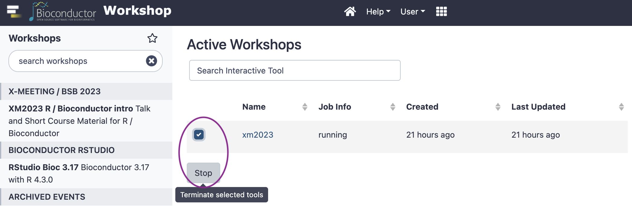
Already have a workshop? STOP IT
-
Choose ‘Active workshops’ from the ‘User’ dropdown

-
Select the existing workshop, and click the ‘Stop’ button
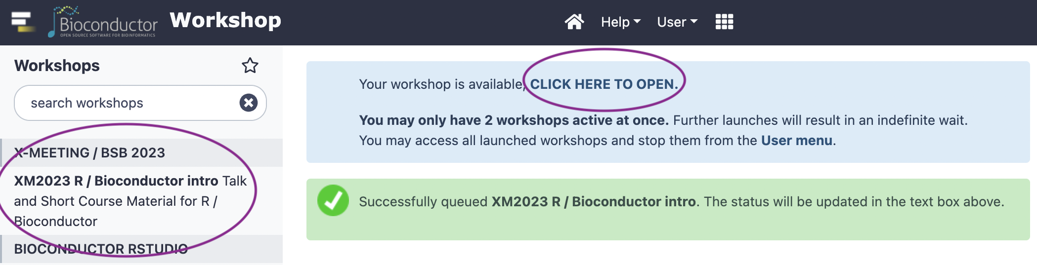
Start a new workshop
choose the ‘X-MEETING / BBS 2023’
Wait a minute or so
Click to open RStudio
-
In RStudio, choose ‘File’ / ‘Open File…’ / ‘vignettes/c_course_part_2.Rmd’
Introduction
This workshop introduces R as an essential tool in
exploratory analysis of bioinformatic data. No previous experience with
R is required. We start with a very short introduction to
R, mentioning vectors, functions, and the
data.frame for representing tabular data. We explore some
essential data management tasks, for instance summarizing cell types and
plotting a ‘UMAP’ in a single-cell RNASeq experiment. We adopt the
‘tidy’ paradigm, using the dplyr package for
data management and ggplot2 for data
visualization. The workshop concludes with a short tour of approaches to
enhance reproducible research in our day-to-day work.
Essential R
A simple calculator
1 + 1
## [1] 2
‘Vectors’ as building blocks
c(1, 2, 3)
## [1] 1 2 3
c("January", "February", "March")
## [1] "January"  "February" "March"
c(TRUE, FALSE)
## [1]  TRUE FALSE
Variables, missing values and ‘factors’
age <- c(27, NA, 32, 29)
gender <- factor(
    c("Female", "Male", "Non-binary", NA),
    levels = c("Female", "Male", "Non-binary")
)
Data structures to coordinate related vectors – the
data.frame
df <- data.frame(
    age = c(27, NA, 32, 29),
    gender = gender
)
df
##   age     gender
## 1  27     Female
## 2  NA       Male
## 3  32 Non-binary
## 4  29       <NA>
Key opererations on data.frame
-
df[1:3, c("gender", "age")]– subset on rows and columns -
df[["age"]],df$age– select columns
Functions
rnorm(5)        # 5 random normal deviates
## [1]  1.27768871 -0.94300715 -0.27247463 -0.53228808  0.07128288
x <- rnorm(100) # 100 random normal deviates
hist(x)         # histogram, approximately normal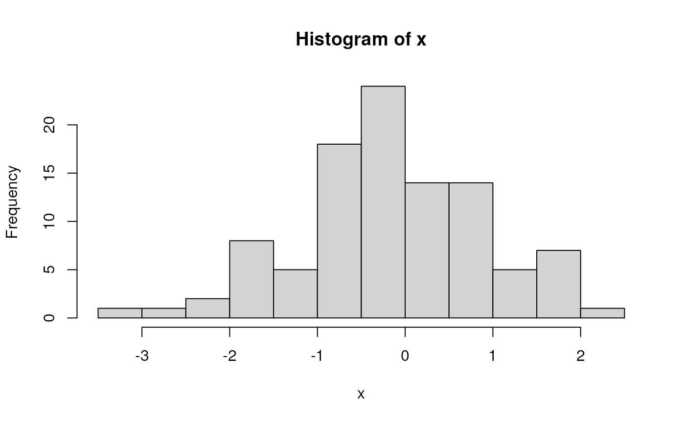

‘Vectorized’ operations, e.g., element-wise addition without an explicit ‘for’ loop
y <- x + rnorm(100)
plot(y ~ x)
fit <- lm(y ~ x)
fit         # an R 'object' containing information about the
##
## Call:
## lm(formula = y ~ x)
##
## Coefficients:
## (Intercept)            x
##    -0.03005      0.97031
            # regression of y on x
abline(fit) # plot points and fitted regression line
anova(fit)  # statistical summary of linear regression
## Analysis of Variance Table
##
## Response: y
##           Df Sum Sq Mean Sq F value    Pr(>F)
## x          1 105.01 105.007  94.944 4.353e-16 ***
## Residuals 98 108.39   1.106
## ---
## Signif. codes:  0 '***' 0.001 '**' 0.01 '*' 0.05 '.' 0.1 ' ' 1
Write your own functions
hello <- function(who) {
    paste("hello", who, "with", nchar(who), "letters in your name")
}
hello("Martin")
## [1] "hello Martin with 6 letters in your name"
Iterate, usually with lapply() although
for() is available
Packages
Extend functionality of base R. Can be part of the ‘base’ distribution…
## iterate over the numbers 1 through 8, 'sleeping' for 1 second
## each. Takes about 8 seconds...
system.time({
    lapply(1:8, function(i) Sys.sleep(1))
})
##    user  system elapsed
##   0.002   0.000   8.010

## sleep in parallel -- takes only 2 seconds
library(parallel)
cl <- makeCluster(4) # cluster of 4 workers
system.time({
    parLapply(cl, 1:8, function(i) Sys.sleep(1))
})
##    user  system elapsed
##   0.003   0.000   2.083
… or a package contributed by users to the Comprehensive R Archive Network (CRAN), or to Bioconductor or other repositories.
Tidyverse
The dplyr contributed CRAN package introduces the ‘tidyverse’
A ‘tibble’ is like a ‘data.frame’, but more user-friendly
tbl <- tibble(
    x = rnorm(100),
    y = x + rnorm(100)
)

## e.g., only displays the first 10 rows
tbl
## # A tibble: 100 × 2
##         x      y
##     <dbl>  <dbl>
##  1  1.55   1.02
##  2 -0.298 -1.72
##  3 -0.350  0.290
##  4  0.673  1.47
##  5  1.23   0.146
##  6 -0.520 -0.664
##  7  0.448 -0.624
##  8 -1.90  -1.56
##  9  1.76   1.32
## 10  0.816  0.409
## # ℹ 90 more rows
The tidyverse makes use of ‘pipes’ |> (the older
syntax is %>%). A pipe takes the left-hand side and pass
through to the right-hand side. Key dplyr ‘verbs’ can be
piped together
-
tibble()– representation of adata.frame, with better display of long and wide data frames.tribble()constructs a tibble in a way that makes the relationship between data across rows more transparent. -
glimpse()– providing a quick look into the columns and data in the tibble by transposing the tibble and display each ‘column’ on a single line. -
select()– column selection. -
filter(),slice()– row selection. -
pull()– extract a single column as a vector. -
mutate()– column transformation. -
count()– count occurences in one or more columns. -
arrange()– order rows by values in one or more columns. -
distinct()– reduce a tibble to only unique rows. -
group_by()– perform computations on groups defined by one or several columns. -
summarize()– calculate summary statstics for groups. -
left_join(),right_join(),inner_join()– merge two tibbles based on shared columns, preserving all rows in the first (left_join()) or second (right_join()) or both (inner_join()) tibble.
tbl |>
    ## e.g., just rows with non-negative values of x and y
    filter(x > 0, y > 0) |>
    ## add a column
    mutate(distance_from_origin = sqrt(x^2 + y^2))
## # A tibble: 41 × 3
##        x     y distance_from_origin
##    <dbl> <dbl>                <dbl>
##  1 1.55  1.02                 1.85
##  2 0.673 1.47                 1.62
##  3 1.23  0.146                1.24
##  4 1.76  1.32                 2.20
##  5 0.816 0.409                0.913
##  6 1.40  1.79                 2.27
##  7 0.910 2.08                 2.27
##  8 0.489 2.78                 2.82
##  9 2.28  2.65                 3.50
## 10 0.132 0.357                0.380
## # ℹ 31 more rows
A ‘classic’ built-in data set – Motor Trend ‘cars’ from 1974…
‘tidyverse’ eschews rownames, so make these a column. Use
group_by() to summarize by group (cyl).
n() is a function from dplyr that returns the number of
records in a group.
mtcars_tbl <-
    mtcars |>
    as_tibble(rownames = "model") |>
    mutate(cyl = factor(cyl))
mtcars_tbl
## # A tibble: 32 × 12
##    model         mpg cyl    disp    hp  drat    wt  qsec    vs    am  gear  carb
##    <chr>       <dbl> <fct> <dbl> <dbl> <dbl> <dbl> <dbl> <dbl> <dbl> <dbl> <dbl>
##  1 Mazda RX4    21   6      160    110  3.9   2.62  16.5     0     1     4     4
##  2 Mazda RX4 …  21   6      160    110  3.9   2.88  17.0     0     1     4     4
##  3 Datsun 710   22.8 4      108     93  3.85  2.32  18.6     1     1     4     1
##  4 Hornet 4 D…  21.4 6      258    110  3.08  3.22  19.4     1     0     3     1
##  5 Hornet Spo…  18.7 8      360    175  3.15  3.44  17.0     0     0     3     2
##  6 Valiant      18.1 6      225    105  2.76  3.46  20.2     1     0     3     1
##  7 Duster 360   14.3 8      360    245  3.21  3.57  15.8     0     0     3     4
##  8 Merc 240D    24.4 4      147.    62  3.69  3.19  20       1     0     4     2
##  9 Merc 230     22.8 4      141.    95  3.92  3.15  22.9     1     0     4     2
## 10 Merc 280     19.2 6      168.   123  3.92  3.44  18.3     1     0     4     4
## # ℹ 22 more rows

mtcars_tbl |>
    group_by(cyl) |>
    summarize(
        n = n(),
        mean_mpg = mean(mpg, na.rm = TRUE),
        var_mpg = var(mpg, na.rm = TRUE)
    )
## # A tibble: 3 × 4
##   cyl       n mean_mpg var_mpg
##   <fct> <int>    <dbl>   <dbl>
## 1 4        11     26.7   20.3
## 2 6         7     19.7    2.11
## 3 8        14     15.1    6.55
Visualization
Another example of a contributed package is ggplot2 for visualization
library(ggplot2)
ggplot(tbl) +
    aes(x, y) +                # use 'x' and 'y' columns for plotting...
    geom_point() +             # ...plot points...
    geom_smooth(method = "lm") # ...linear regresion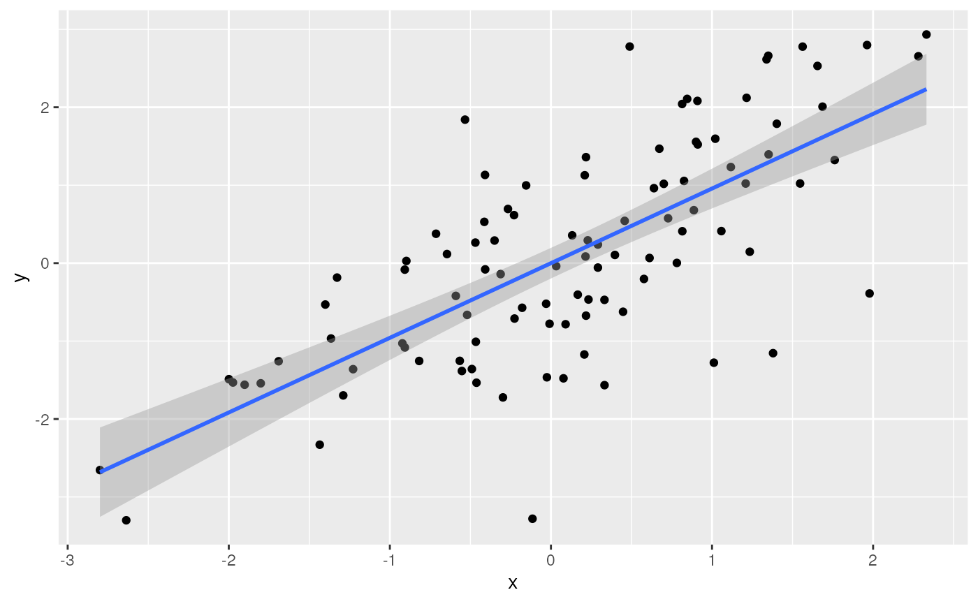
Check out plotly, especially for interactive visualization (e.g., ‘tooltips’ when mousing over points, or dragging to subset and zoom in)
library(plotly)
plt <-
    ggplot(mtcars_tbl) +
    aes(x = cyl, y = mpg, text = model) +
    geom_jitter(width = .25) +
    geom_boxplot()
ggplotly(plt)
Where do Packages Come From?
CRAN: Comprehensive R Archive Network. More than 18,000 packages. Some help from CRAN Task Views in identifying relevant packages.
Bioconductor: More than 2100 packages relevant to high-throughput genomic analysis. Vignettes are an important part of Bioconductor packages.
Install packages once per R installation, using
BiocManager::install(<package-name>) (CRAN or
Bioconductor)
What about GitHub? Packages haven’t been checked by a formal system, so may have incomplete code, documentation, dependencies on other packages, etc. Authors may not yet be committed to long-term maintenance of their package.
Bioinformatics – scRNA-seq
Cell summary
Read a ‘csv’ file summarizing infomration about each cell in the experiment.
## use `file.choose()` or similar for your own data sets
cell_data_csv <- system.file(package = "XM2023", "scrnaseq-cell-data.csv")
cell_data <- readr::read_csv(cell_data_csv)
cell_data |>
    glimpse()
## Rows: 31,696
## Columns: 37
## $ cell_id                                  <chr> "CMGpool_AAACCCAAGGACAACC", "…
## $ UMAP_1                                   <dbl> -5.9931696, -6.7217583, -9.01…
## $ UMAP_2                                   <dbl> -1.9311870, -1.3059803, -3.39…
## $ donor_id                                 <chr> "pooled [D9,D7,D8,D10,D6]", "…
## $ self_reported_ethnicity_ontology_term_id <chr> "HANCESTRO:0005", "HANCESTRO:…
## $ donor_BMI                                <chr> "pooled [30.5,22.7,23.5,26.8,…
## $ donor_times_pregnant                     <chr> "pooled [3,0,3,2,2]", "pooled…
## $ family_history_breast_cancer             <chr> "pooled [unknown,False,False,…
## $ organism_ontology_term_id                <chr> "NCBITaxon:9606", "NCBITaxon:…
## $ tyrer_cuzick_lifetime_risk               <chr> "pooled [12,14.8,8.8,14.3,20.…
## $ sample_uuid                              <chr> "pooled [f008c67a-abb4-4563-8…
## $ sample_preservation_method               <chr> "cryopreservation", "cryopres…
## $ tissue_ontology_term_id                  <chr> "UBERON:0035328", "UBERON:003…
## $ development_stage_ontology_term_id       <chr> "HsapDv:0000087", "HsapDv:000…
## $ suspension_uuid                          <chr> "38d793cb-d811-4863-aec0-2fa7…
## $ suspension_type                          <chr> "cell", "cell", "cell", "cell…
## $ library_uuid                             <chr> "385d8d7c-5038-4f0e-b7f3-ec9a…
## $ assay_ontology_term_id                   <chr> "EFO:0009922", "EFO:0009922",…
## $ mapped_reference_annotation              <chr> "GENCODE 28", "GENCODE 28", "…
## $ is_primary_data                          <lgl> TRUE, TRUE, TRUE, TRUE, TRUE,…
## $ cell_type_ontology_term_id               <chr> "CL:0011026", "CL:0011026", "…
## $ author_cell_type                         <chr> "luminal progenitor", "lumina…
## $ disease_ontology_term_id                 <chr> "PATO:0000461", "PATO:0000461…
## $ sex_ontology_term_id                     <chr> "PATO:0000383", "PATO:0000383…
## $ nCount_RNA                               <dbl> 2937, 5495, 5598, 3775, 2146,…
## $ nFeature_RNA                             <dbl> 1183, 1827, 2037, 1448, 1027,…
## $ percent.mito                             <dbl> 0.02076949, 0.03676069, 0.043…
## $ seurat_clusters                          <dbl> 3, 3, 24, 1, 3, 1, 1, 4, 1, 0…
## $ sample_id                                <chr> "CMGpool", "CMGpool", "CMGpoo…
## $ cell_type                                <chr> "progenitor cell", "progenito…
## $ assay                                    <chr> "10x 3' v3", "10x 3' v3", "10…
## $ disease                                  <chr> "normal", "normal", "normal",…
## $ organism                                 <chr> "Homo sapiens", "Homo sapiens…
## $ sex                                      <chr> "female", "female", "female",…
## $ tissue                                   <chr> "upper outer quadrant of brea…
## $ self_reported_ethnicity                  <chr> "European", "European", "Euro…
## $ development_stage                        <chr> "human adult stage", "human a…
Summarize information – how many donors, what developmental stage, what ethnicity?
cell_data |>
    count(donor_id, development_stage, self_reported_ethnicity)
## # A tibble: 7 × 4
##   donor_id                 development_stage       self_reported_ethnicity     n
##   <chr>                    <chr>                   <chr>                   <int>
## 1 D1                       35-year-old human stage European                 2303
## 2 D11                      43-year-old human stage Chinese                  7454
## 3 D2                       60-year-old human stage European                  864
## 4 D3                       44-year-old human stage African American         2517
## 5 D4                       42-year-old human stage European                 1771
## 6 D5                       21-year-old human stage European                 2244
## 7 pooled [D9,D7,D8,D10,D6] human adult stage       European                14543
What cell types have been annotated?
cell_data |>
    count(cell_type)
## # A tibble: 6 × 2
##   cell_type                                    n
##   <chr>                                    <int>
## 1 B cell                                     215
## 2 basal cell                                7040
## 3 endocrine cell                              64
## 4 endothelial cell of lymphatic vessel       133
## 5 luminal epithelial cell of mammary gland  4257
## 6 progenitor cell                          19987
Cell types for each ethnicity?
cell_data |>
    count(self_reported_ethnicity, cell_type) |>
    tidyr::pivot_wider(
               names_from = "self_reported_ethnicity",
               values_from = "n"
           )
## # A tibble: 6 × 4
##   cell_type                                `African American` Chinese European
##   <chr>                                                 <int>   <int>    <int>
## 1 B cell                                                    5      73      137
## 2 basal cell                                              583    3367     3090
## 3 endothelial cell of lymphatic vessel                     11      31       91
## 4 luminal epithelial cell of mammary gland                809     187     3261
## 5 progenitor cell                                        1109    3755    15123
## 6 endocrine cell                                           NA      41       23
Reflecting on this – there is no replication across non-European ethnicity, so no statistical insights available. Pooled samples probably require careful treatment in any downstream analysis.
UMAP visualization
Use the ‘UMAP’ columns to visualize gene expression
library(ggplot2)
plt <-
    ggplot(cell_data) +
    aes(UMAP_1, UMAP_2, color = cell_type) +
    geom_point(pch = ".")
plt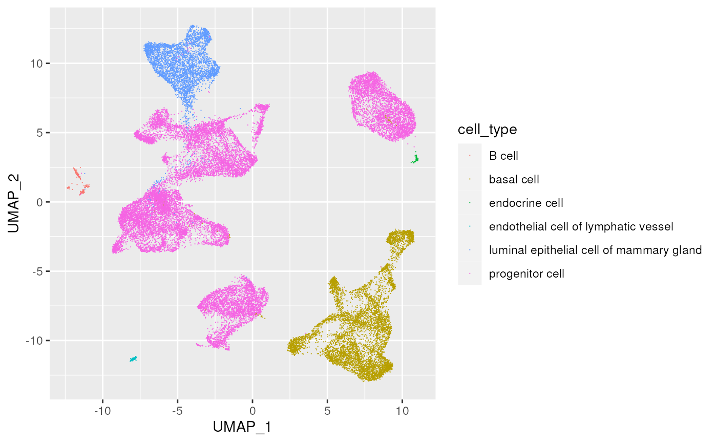
Make this interactive, for mouse-over ‘tool tips’ and ‘brushing’ selection
Genes
## use `file.choose()` or similar for your own data sets
row_data_csv <- system.file(package = "XM2023", "scrnaseq-gene-data.csv")
row_data <- readr::read_csv(row_data_csv)
row_data |>
    glimpse()
## Rows: 33,234
## Columns: 7
## $ gene_id             <chr> "ENSG00000243485", "ENSG00000237613", "ENSG0000018…
## $ feature_is_filtered <lgl> TRUE, TRUE, TRUE, FALSE, TRUE, TRUE, TRUE, TRUE, T…
## $ feature_name        <chr> "MIR1302-2HG", "FAM138A", "OR4F5", "RP11-34P13.7",…
## $ feature_reference   <chr> "NCBITaxon:9606", "NCBITaxon:9606", "NCBITaxon:960…
## $ feature_biotype     <chr> "gene", "gene", "gene", "gene", "gene", "gene", "g…
## $ mean_expression     <dbl> 3.154972e-05, 0.000000e+00, 0.000000e+00, 2.208481…
## $ mean_log_expression <dbl> 0.0000218686, 0.0000000000, 0.0000000000, 0.001521…
Approximately 1/3rd have been flagged to be filtered. All genes are
from humans (NCBITaxon:9606) and are of biotype ‘gene’.
row_data |>
    count(feature_is_filtered, feature_reference, feature_biotype)
## # A tibble: 2 × 4
##   feature_is_filtered feature_reference feature_biotype     n
##   <lgl>               <chr>             <chr>           <int>
## 1 FALSE               NCBITaxon:9606    gene            22743
## 2 TRUE                NCBITaxon:9606    gene            10491
A simple plot shows the distribution of log-transformed average expression of each gene
row_data |>
    filter(!feature_is_filtered) |>
    ggplot() +
    aes(x = mean_log_expression) +
    geom_histogram()
## `stat_bin()` using `bins = 30`. Pick better value with `binwidth`.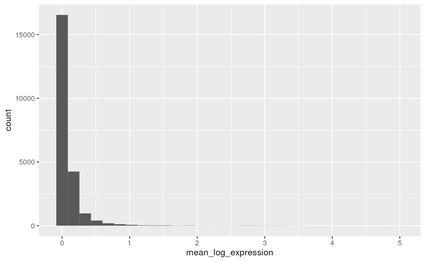
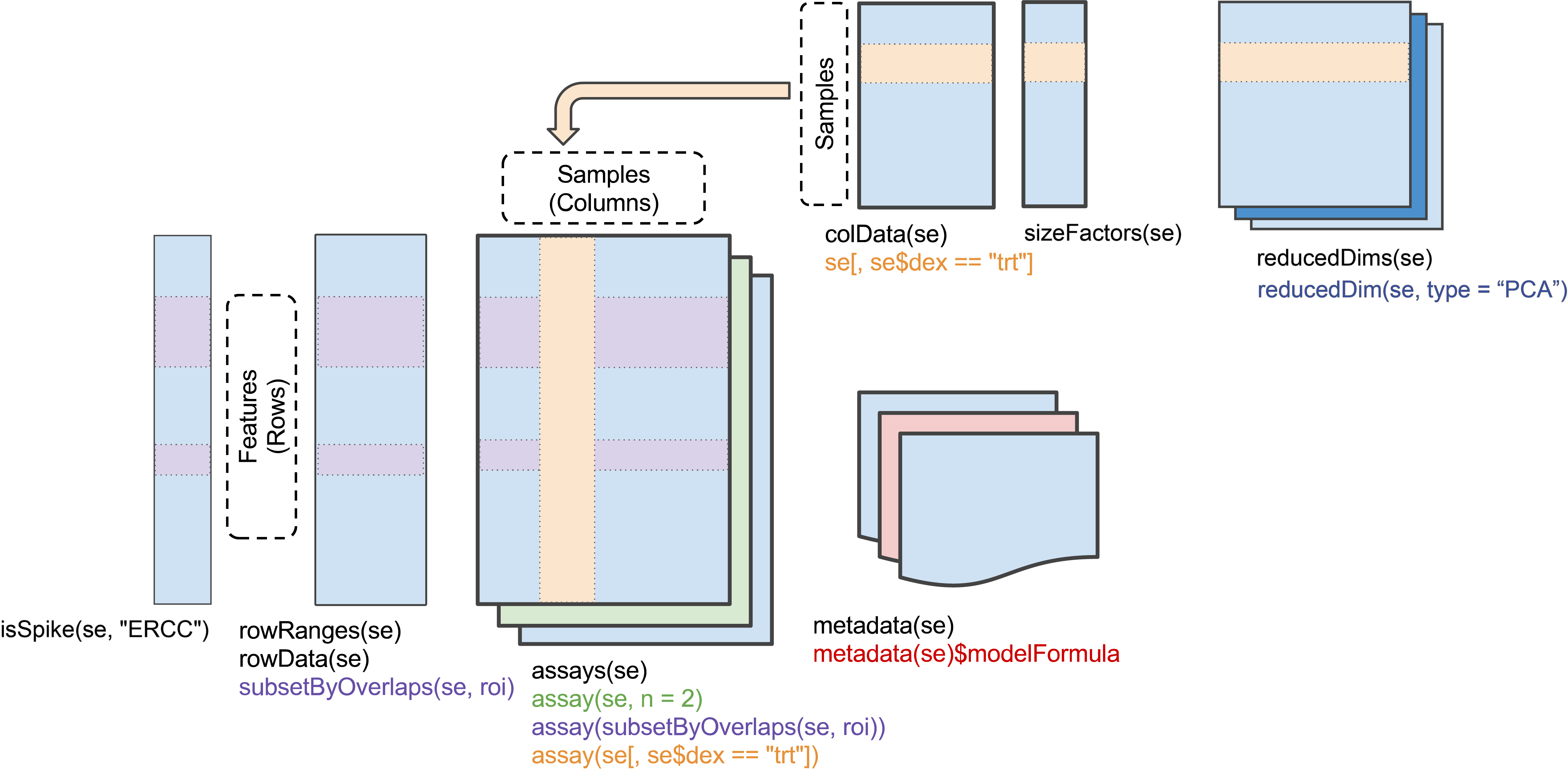
SingleCellExperiment
Row (gene) data, column (cell) data, and a matrix of counts describe
a single cell experiment. These can be assembled, along with other
information about, e.g., reduced dimension representations, into a
‘SingleCellExperiment’ Bioconductor object (see
?SingleCellExperiment).
Here we illustrate this construction with some artificial data:
library(SingleCellExperiment)

n_genes <- 200
n_cells <- 100

demo_count <- matrix(rpois(20000, 5), ncol=n_cells) # counts
demo_log_count <- log2(demo_count + 1)              # log counts

demo_row_data <- data.frame(
    gene_id = paste0("gene_", seq_len(n_genes))
)
demo_column_data <- data.frame(
    cell_id = paste0("cell_", seq_len(n_cells))
)

demo_pca <- matrix(runif(n_cells * 5), n_cells)
demo_tsne <- matrix(rnorm(n_cells * 2), n_cells)
demo_sce <- SingleCellExperiment(
    assays=list(counts=demo_count, logcounts=demo_log_count),
    colData = demo_column_data,
    rowData = demo_row_data,
    reducedDims=SimpleList(PCA=demo_pca, tSNE=demo_tsne)
)
demo_sce
## class: SingleCellExperiment
## dim: 200 100
## metadata(0):
## assays(2): counts logcounts
## rownames: NULL
## rowData names(1): gene_id
## colnames: NULL
## colData names(1): cell_id
## reducedDimNames(2): PCA tSNE
## mainExpName: NULL
## altExpNames(0):
Elements of the object can be obtained using ’accessors`, e.g.,
Bioconductor resources
Overview
Web site – https://bioconductor.org
- Available packages https://bioconductor.org/packages
- Package landing pages & vignettes, e.g., https://bioconductor.org/packages/scater
Package installation
- Use CRAN package BiocManager
- Bioconductor, CRAN, and github packages
if (!"BiocManager" %in% rownames(installed.packages()))
    install.packages("BiocManager", repos = "https://cran.R-project.org")
BiocManager::install("GenomicFeatures")
Support site – https://support.bioconductor.org
- also
- slack – sign up - https://slack.bioconductor.org/
- Bug reports, e.g.,
bug.report(package = "GenomicFeatures") - direct email to maintainers
maintainer("GenomicFeatures")
Source code
-
git clone https://git.bioconductor.org/packages/GenomicFeatures
Other resources
Annotations
From row_data, we know each Ensembl gene id, but what
else can we learn about these genes?
library(AnnotationHub)
ah <- AnnotationHub()
query(ah, c("EnsDb", "Homo sapiens"))
## AnnotationHub with 24 records
## # snapshotDate(): 2023-05-15
## # $dataprovider: Ensembl
## # $species: Homo sapiens
## # $rdataclass: EnsDb
## # additional mcols(): taxonomyid, genome, description,
## #   coordinate_1_based, maintainer, rdatadateadded, preparerclass, tags,
## #   rdatapath, sourceurl, sourcetype
## # retrieve records with, e.g., 'object[["AH53211"]]'
##
##              title
##   AH53211  | Ensembl 87 EnsDb for Homo Sapiens
##   AH53715  | Ensembl 88 EnsDb for Homo Sapiens
##   AH56681  | Ensembl 89 EnsDb for Homo Sapiens
##   AH57757  | Ensembl 90 EnsDb for Homo Sapiens
##   AH60773  | Ensembl 91 EnsDb for Homo Sapiens
##   ...        ...
##   AH98047  | Ensembl 105 EnsDb for Homo sapiens
##   AH100643 | Ensembl 106 EnsDb for Homo sapiens
##   AH104864 | Ensembl 107 EnsDb for Homo sapiens
##   AH109336 | Ensembl 108 EnsDb for Homo sapiens
##   AH109606 | Ensembl 109 EnsDb for Homo sapiens
ensdb109 <- ah[["AH109606"]]
## loading from cache
## require("ensembldb")
ensdb109
## EnsDb for Ensembl:
## |Backend: SQLite
## |Db type: EnsDb
## |Type of Gene ID: Ensembl Gene ID
## |Supporting package: ensembldb
## |Db created by: ensembldb package from Bioconductor
## |script_version: 0.3.10
## |Creation time: Thu Feb 16 12:36:05 2023
## |ensembl_version: 109
## |ensembl_host: localhost
## |Organism: Homo sapiens
## |taxonomy_id: 9606
## |genome_build: GRCh38
## |DBSCHEMAVERSION: 2.2
## |common_name: human
## |species: homo_sapiens
## | No. of genes: 70623.
## | No. of transcripts: 276218.
## |Protein data available.
There are a number of ‘tables’ of data in the EnsDb; check out
browseVignettes("ensembldb") for more information.
names(listTables(ensdb109))
##  [1] "gene"           "tx"             "tx2exon"        "exon"
##  [5] "chromosome"     "protein"        "uniprot"        "protein_domain"
##  [9] "entrezgene"     "metadata"
E.g., add information about each unfiltered gene from
row_data.
-
get gene annotations from the EnsDB object
gene_annotations <- genes( ensdb109, filter = ~ gene_biotype == "protein_coding", return.type = "DataFrame" ) |> as_tibble() gene_annotations ## # A tibble: 22,907 × 13 ## gene_id gene_name gene_biotype gene_seq_start gene_seq_end seq_name ## <chr> <chr> <chr> <int> <int> <chr> ## 1 ENSG00000186092 OR4F5 protein_coding 65419 71585 1 ## 2 ENSG00000284733 OR4F29 protein_coding 450740 451678 1 ## 3 ENSG00000284662 OR4F16 protein_coding 685716 686654 1 ## 4 ENSG00000187634 SAMD11 protein_coding 923923 944575 1 ## 5 ENSG00000188976 NOC2L protein_coding 944203 959309 1 ## 6 ENSG00000187961 KLHL17 protein_coding 960584 965719 1 ## 7 ENSG00000187583 PLEKHN1 protein_coding 966482 975865 1 ## 8 ENSG00000187642 PERM1 protein_coding 975198 982117 1 ## 9 ENSG00000188290 HES4 protein_coding 998962 1000172 1 ## 10 ENSG00000187608 ISG15 protein_coding 1001138 1014540 1 ## # ℹ 22,897 more rows ## # ℹ 7 more variables: seq_strand <int>, seq_coord_system <chr>, ## # description <chr>, gene_id_version <chr>, canonical_transcript <chr>, ## # symbol <chr>, entrezid <named list> -
left_join()the filteredrow_datatogene_annotations(i.e., keep all rows from the filtered row data, and add columns for matching rows fromgene_annotations)row_data |> dplyr::filter(!feature_is_filtered) |> left_join(gene_annotations) ## Joining with `by = join_by(gene_id)` ## # A tibble: 22,743 × 19 ## gene_id feature_is_filtered feature_name feature_reference feature_biotype ## <chr> <lgl> <chr> <chr> <chr> ## 1 ENSG00000… FALSE RP11-34P13.7 NCBITaxon:9606 gene ## 2 ENSG00000… FALSE LINC01409 NCBITaxon:9606 gene ## 3 ENSG00000… FALSE FAM87B NCBITaxon:9606 gene ## 4 ENSG00000… FALSE LINC00115 NCBITaxon:9606 gene ## 5 ENSG00000… FALSE FAM41C NCBITaxon:9606 gene ## 6 ENSG00000… FALSE RP11-54O7.1 NCBITaxon:9606 gene ## 7 ENSG00000… FALSE LINC02593 NCBITaxon:9606 gene ## 8 ENSG00000… FALSE SAMD11 NCBITaxon:9606 gene ## 9 ENSG00000… FALSE NOC2L NCBITaxon:9606 gene ## 10 ENSG00000… FALSE KLHL17 NCBITaxon:9606 gene ## # ℹ 22,733 more rows ## # ℹ 14 more variables: mean_expression <dbl>, mean_log_expression <dbl>, ## # gene_name <chr>, gene_biotype <chr>, gene_seq_start <int>, ## # gene_seq_end <int>, seq_name <chr>, seq_strand <int>, ## # seq_coord_system <chr>, description <chr>, gene_id_version <chr>, ## # canonical_transcript <chr>, symbol <chr>, entrezid <named list>
Many other annotation resources available, to help place information about genes into biological context.
Experiments
Bioconductor provides ‘experiment’ data in addition to software packages and annotation resources. Experiment data includes datasets used for training and other purposes; they are often made available through a package.
Load the MouseGastrulationData package and an example single cell experiment
library(MouseGastrulationData)
sce <- WTChimeraData(samples=5:10)
sce
## class: SingleCellExperiment
## dim: 29453 20935
## metadata(0):
## assays(1): counts
## rownames(29453): ENSMUSG00000051951 ENSMUSG00000089699 ...
##   ENSMUSG00000095742 tomato-td
## rowData names(2): ENSEMBL SYMBOL
## colnames(20935): cell_9769 cell_9770 ... cell_30702 cell_30703
## colData names(11): cell barcode ... doub.density sizeFactor
## reducedDimNames(2): pca.corrected.E7.5 pca.corrected.E8.5
## mainExpName: NULL
## altExpNames(0):
Use colData() and dplyr to explore cell annotations
colData(sce)
## DataFrame with 20935 rows and 11 columns
## cell barcode sample stage tomato
## <character> <character> <integer> <character> <logical>
## cell_9769 cell_9769 AAACCTGAGACTGTAA 5 E8.5 TRUE
## cell_9770 cell_9770 AAACCTGAGATGCCTT 5 E8.5 TRUE
## cell_9771 cell_9771 AAACCTGAGCAGCCTC 5 E8.5 TRUE
## cell_9772 cell_9772 AAACCTGCATACTCTT 5 E8.5 TRUE
## cell_9773 cell_9773 AAACGGGTCAACACCA 5 E8.5 TRUE
## ... ... ... ... ... ...
## cell_30699 cell_30699 TTTGTCACAGCTCGCA 10 E8.5 FALSE
## cell_30700 cell_30700 TTTGTCAGTCTAGTCA 10 E8.5 FALSE
## cell_30701 cell_30701 TTTGTCATCATCGGAT 10 E8.5 FALSE
## cell_30702 cell_30702 TTTGTCATCATTATCC 10 E8.5 FALSE
## cell_30703 cell_30703 TTTGTCATCCCATTTA 10 E8.5 FALSE
## pool stage.mapped celltype.mapped closest.cell
## <integer> <character> <character> <character>
## cell_9769 3 E8.25 Mesenchyme cell_24159
## cell_9770 3 E8.5 Endothelium cell_96660
## cell_9771 3 E8.5 Allantois cell_134982
## cell_9772 3 E8.5 Erythroid3 cell_133892
## cell_9773 3 E8.25 Erythroid1 cell_76296
## ... ... ... ... ...
## cell_30699 5 E8.5 Erythroid3 cell_38810
## cell_30700 5 E8.5 Surface ectoderm cell_38588
## cell_30701 5 E8.25 Forebrain/Midbrain/H.. cell_66082
## cell_30702 5 E8.5 Erythroid3 cell_138114
## cell_30703 5 E8.0 Doublet cell_92644
## doub.density sizeFactor
## <numeric> <numeric>
## cell_9769 0.02985045 1.41243
## cell_9770 0.00172753 1.22757
## cell_9771 0.01338013 1.15439
## cell_9772 0.00218402 1.28676
## cell_9773 0.00211723 1.78719
## ... ... ...
## cell_30699 0.00146287 0.389311
## cell_30700 0.00374155 0.588784
## cell_30701 0.05651258 0.624455
## cell_30702 0.00108837 0.550807
## cell_30703 0.82369305 1.184919
colData(sce) |>
dplyr::as_tibble() |>
dplyr::count(sample)
## # A tibble: 6 × 2
## sample n
## <int> <int>
## 1 5 2411
## 2 6 1047
## 3 7 3007
## 4 8 3097
## 5 9 4544
## 6 10 6829
colData(sce) |>
dplyr::as_tibble() |>
dplyr::count(celltype.mapped)
## # A tibble: 35 × 2
## celltype.mapped n
## <chr> <int>
## 1 Allantois 955
## 2 Blood progenitors 1 56
## 3 Blood progenitors 2 245
## 4 Cardiomyocytes 601
## 5 Caudal Mesoderm 71
## 6 Caudal epiblast 71
## 7 Caudal neurectoderm 19
## 8 Def. endoderm 91
## 9 Doublet 1509
## 10 Endothelium 350
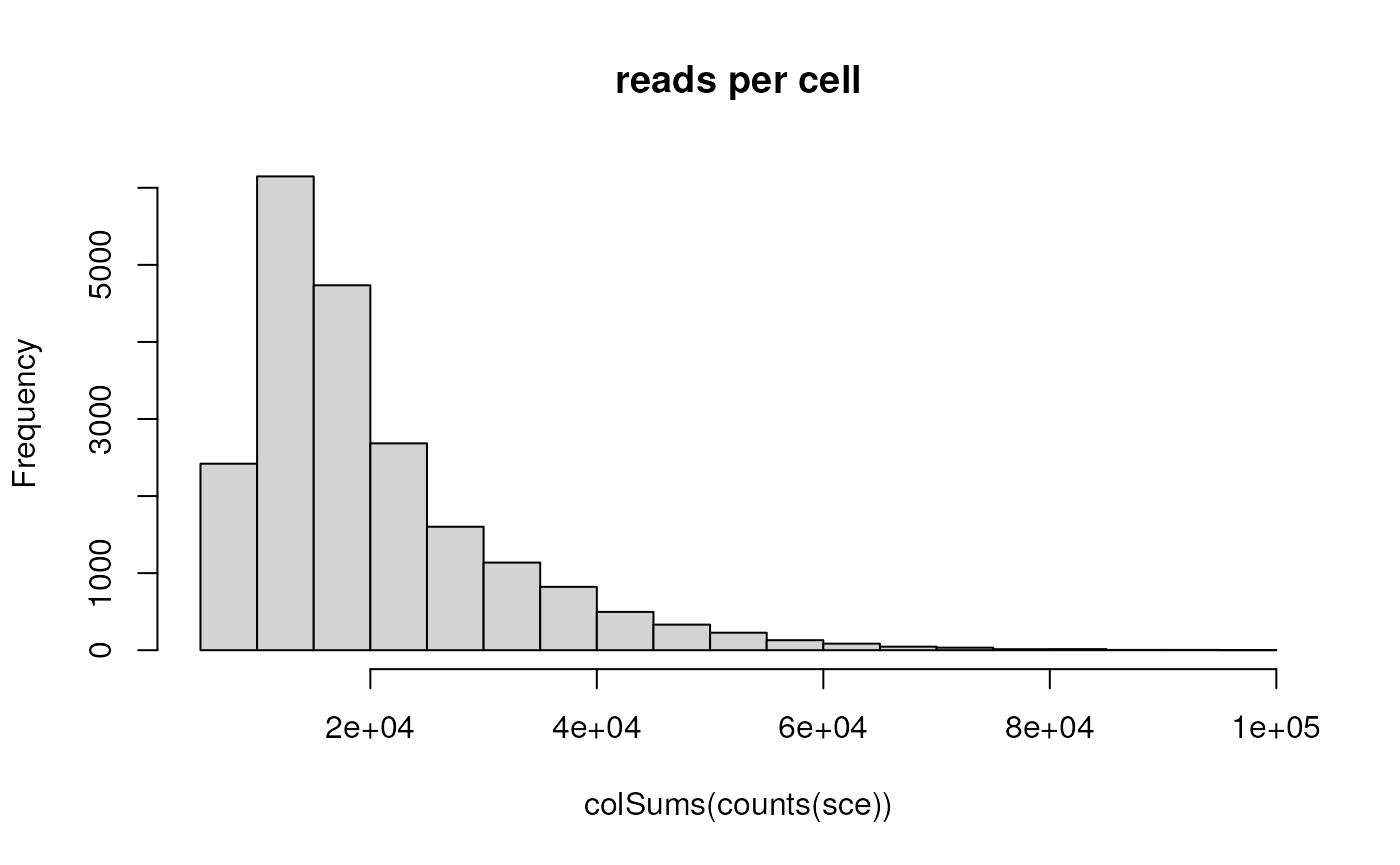
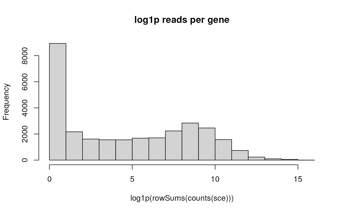
## # ℹ 25 more rowsUse the counts() accessor to obtain the genes x cells
matrix of counts of reads mapped to each gene. Use
colSums() and the base graphics hist() to
summarize the number of reads per cell.
Likewise for summarizing log + 1 reads per gene, using ‘pipes’
The row data contains just Ensembl and gene symbol annotations. From the ‘MouseGastrulationData’ vignette, this experiment used Ensembl mouse annotations, version 92. Discover and retrieve these annotations using AnnotationHub
## Ensembl 92 genome annotation
library(AnnotationHub)
ah <- AnnotationHub()
query(ah, c("EnsDb", "Mus musculus", "92"))
## AnnotationHub with 2 records
## # snapshotDate(): 2023-05-15
## # $dataprovider: Ensembl
## # $species: Mus musculus domesticus, Mus musculus
## # $rdataclass: EnsDb
## # additional mcols(): taxonomyid, genome, description,
## #   coordinate_1_based, maintainer, rdatadateadded, preparerclass, tags,
## #   rdatapath, sourceurl, sourcetype
## # retrieve records with, e.g., 'object[["AH60992"]]'
##
##              title
##   AH60992  | Ensembl 92 EnsDb for Mus Musculus
##   AH109654 | Ensembl 109 EnsDb for Mus musculus domesticus
edb <- ah[["AH60992"]]
## loading from cache
Check out the ensembldb vignette. Retrieve additional annotations available on genes
genes(edb)
## GRanges object with 54590 ranges and 8 metadata columns:
##                      seqnames            ranges strand |            gene_id
##                         <Rle>         <IRanges>  <Rle> |        <character>
##   ENSMUSG00000102693        1   3073253-3074322      + | ENSMUSG00000102693
##   ENSMUSG00000064842        1   3102016-3102125      + | ENSMUSG00000064842
##   ENSMUSG00000051951        1   3205901-3671498      - | ENSMUSG00000051951
##   ENSMUSG00000102851        1   3252757-3253236      + | ENSMUSG00000102851
##   ENSMUSG00000103377        1   3365731-3368549      - | ENSMUSG00000103377
##                  ...      ...               ...    ... .                ...
##   ENSMUSG00000095134        Y 90753057-90763485      + | ENSMUSG00000095134
##   ENSMUSG00000095366        Y 90754513-90754821      - | ENSMUSG00000095366
##   ENSMUSG00000096768        Y 90784738-90816464      + | ENSMUSG00000096768
##   ENSMUSG00000099871        Y 90837413-90844040      + | ENSMUSG00000099871
##   ENSMUSG00000096850        Y 90838869-90839177      - | ENSMUSG00000096850
##                          gene_name           gene_biotype seq_coord_system
##                        <character>            <character>      <character>
##   ENSMUSG00000102693 4933401J01Rik                    TEC       chromosome
##   ENSMUSG00000064842       Gm26206                  snRNA       chromosome
##   ENSMUSG00000051951          Xkr4         protein_coding       chromosome
##   ENSMUSG00000102851       Gm18956   processed_pseudogene       chromosome
##   ENSMUSG00000103377       Gm37180                    TEC       chromosome
##                  ...           ...                    ...              ...
##   ENSMUSG00000095134      Mid1-ps1 unprocessed_pseudogene       chromosome
##   ENSMUSG00000095366       Gm21860         protein_coding       chromosome
##   ENSMUSG00000096768       Gm47283         protein_coding       chromosome
##   ENSMUSG00000099871       Gm21742 unprocessed_pseudogene       chromosome
##   ENSMUSG00000096850       Gm21748         protein_coding       chromosome
##                                 description      gene_id_version        symbol
##                                 <character>          <character>   <character>
##   ENSMUSG00000102693 RIKEN cDNA 4933401J0.. ENSMUSG00000102693.1 4933401J01Rik
##   ENSMUSG00000064842 predicted gene, 2620.. ENSMUSG00000064842.1       Gm26206
##   ENSMUSG00000051951 X-linked Kx blood gr.. ENSMUSG00000051951.5          Xkr4
##   ENSMUSG00000102851 predicted gene, 1895.. ENSMUSG00000102851.1       Gm18956
##   ENSMUSG00000103377 predicted gene, 3718.. ENSMUSG00000103377.1       Gm37180
##                  ...                    ...                  ...           ...
##   ENSMUSG00000095134 midline 1, pseudogen.. ENSMUSG00000095134.2      Mid1-ps1
##   ENSMUSG00000095366                   NULL ENSMUSG00000095366.1       Gm21860
##   ENSMUSG00000096768 predicted gene, 4728.. ENSMUSG00000096768.7       Gm47283
##   ENSMUSG00000099871 predicted gene, 2174.. ENSMUSG00000099871.1       Gm21742
##   ENSMUSG00000096850                   NULL ENSMUSG00000096850.1       Gm21748
##                      entrezid
##                        <list>
##   ENSMUSG00000102693     <NA>
##   ENSMUSG00000064842     <NA>
##   ENSMUSG00000051951   497097
##   ENSMUSG00000102851     <NA>
##   ENSMUSG00000103377     <NA>
##                  ...      ...
##   ENSMUSG00000095134     <NA>
##   ENSMUSG00000095366     <NA>
##   ENSMUSG00000096768   170942
##   ENSMUSG00000099871     <NA>
##   ENSMUSG00000096850     <NA>
##   -------
##   seqinfo: 117 sequences (1 circular) from GRCm38 genome
Use a filter to identify genes on chromosome 1, and in the row names
of sce
filter <- list(
    SeqNameFilter("1"),
    AnnotationFilter(~gene_id %in% rownames(sce))
)
chr1 <- genes(edb, filter = filter)
Finally, subset the SingleCellExperiment to contain just genes on chromsoome 1.
sce[names(chr1), ]
## class: SingleCellExperiment
## dim: 1734 20935
## metadata(0):
## assays(1): counts
## rownames(1734): ENSMUSG00000051951 ENSMUSG00000089699 ...
##   ENSMUSG00000016481 ENSMUSG00000026616
## rowData names(2): ENSEMBL SYMBOL
## colnames(20935): cell_9769 cell_9770 ... cell_30702 cell_30703
## colData names(11): cell barcode ... doub.density sizeFactor
## reducedDimNames(2): pca.corrected.E7.5 pca.corrected.E8.5
## mainExpName: NULL
## altExpNames(0):
Reproducibility
Packages
-
Provide a robust way to document requirements for analysis, and to organize complicated analyses into distinct steps.
devtools::create("MyAnalysis") setwd("MyAnalysis") usethis::use_vignette("a_data_management", "A. Data management") usethis::use_vignette("b_exploratory_visualization", "B. Exploration") -
I’ve found pkgdown to be very useful for presenting packages to my users. For instance, material from this workshop is available through pkgdown.
usethis::use_pkgdown()
pkgdown::build_site()
Vignettes
- Explict description of analysis steps (good for the bioinformatician), coupled with text and graphics (good for the collaboration).
Git
- Incremental ‘commits’ as analysis progresses.
- Commits allow confident exploration – the last commit is always available to ‘start over’.
- Tags allow checkpointing an analysis, e.g., the version of the analysis used in the original manuscript submission; the version of the analysis associated with the revision and final publciation.
Containers
- A fully reproducible analysis is very challenging to implement – specifying software version is not enough, and is not easy for a future investigator to re-establish.
- Containers like docker or singularity provide one mechanism for creating a ‘snapshot’ capturing exactly the software used.
- Beware! Complicated containers might result in a fully reproducible analysis, but provide little confidence in the robustness of the analysis.
Summary
More to come…
Tomorrow
- Discover single-cell data sets in the CELLxGENE data portal
- Download and import data sets as ‘Seurat’ or ‘SingleCellExperiment’ objects.
- Coordinate cell annotation and gene annotation
Session information
This document was produced with the following R software:
sessionInfo()
## R version 4.3.0 (2023-04-21)
## Platform: x86_64-pc-linux-gnu (64-bit)
## Running under: Ubuntu 22.04.2 LTS
##
## Matrix products: default
## BLAS:   /usr/lib/x86_64-linux-gnu/openblas-pthread/libblas.so.3
## LAPACK: /usr/lib/x86_64-linux-gnu/openblas-pthread/libopenblasp-r0.3.20.so;  LAPACK version 3.10.0
##
## locale:
##  [1] LC_CTYPE=en_US.UTF-8       LC_NUMERIC=C
##  [3] LC_TIME=en_US.UTF-8        LC_COLLATE=en_US.UTF-8
##  [5] LC_MONETARY=en_US.UTF-8    LC_MESSAGES=en_US.UTF-8
##  [7] LC_PAPER=en_US.UTF-8       LC_NAME=C
##  [9] LC_ADDRESS=C               LC_TELEPHONE=C
## [11] LC_MEASUREMENT=en_US.UTF-8 LC_IDENTIFICATION=C
##
## time zone: Etc/UTC
## tzcode source: system (glibc)
##
## attached base packages:
## [1] stats4    parallel  stats     graphics  grDevices utils     datasets
## [8] methods   base
##
## other attached packages:
##  [1] MouseGastrulationData_1.15.0 SpatialExperiment_1.11.0
##  [3] ensembldb_2.25.0             AnnotationFilter_1.25.0
##  [5] GenomicFeatures_1.53.0       AnnotationDbi_1.63.1
##  [7] AnnotationHub_3.9.1          BiocFileCache_2.9.0
##  [9] dbplyr_2.3.2                 SingleCellExperiment_1.23.0
## [11] SummarizedExperiment_1.31.1  Biobase_2.61.0
## [13] GenomicRanges_1.53.1         GenomeInfoDb_1.37.1
## [15] IRanges_2.35.1               S4Vectors_0.39.1
## [17] BiocGenerics_0.47.0          MatrixGenerics_1.13.0
## [19] matrixStats_1.0.0            plotly_4.10.2
## [21] ggplot2_3.4.2                dplyr_1.1.2
##
## loaded via a namespace (and not attached):
##   [1] jsonlite_1.8.5                magrittr_2.0.3
##   [3] magick_2.7.4                  farver_2.1.1
##   [5] rmarkdown_2.22                fs_1.6.2
##   [7] BiocIO_1.11.0                 zlibbioc_1.47.0
##   [9] ragg_1.2.5                    vctrs_0.6.3
##  [11] DelayedMatrixStats_1.23.0     memoise_2.0.1
##  [13] Rsamtools_2.17.0              RCurl_1.98-1.12
##  [15] htmltools_0.5.5               S4Arrays_1.1.4
##  [17] progress_1.2.2                curl_5.0.1
##  [19] Rhdf5lib_1.23.0               rhdf5_2.45.0
##  [21] SparseArray_1.1.10            sass_0.4.6
##  [23] bslib_0.5.0                   htmlwidgets_1.6.2
##  [25] desc_1.4.2                    cachem_1.0.8
##  [27] GenomicAlignments_1.37.0      mime_0.12
##  [29] lifecycle_1.0.3               pkgconfig_2.0.3
##  [31] Matrix_1.5-4.1                R6_2.5.1
##  [33] fastmap_1.1.1                 GenomeInfoDbData_1.2.10
##  [35] shiny_1.7.4                   digest_0.6.31
##  [37] colorspace_2.1-0              rprojroot_2.0.3
##  [39] dqrng_0.3.0                   ExperimentHub_2.7.1
##  [41] textshaping_0.3.6             crosstalk_1.2.0
##  [43] RSQLite_2.3.1                 beachmat_2.17.8
##  [45] filelock_1.0.2                labeling_0.4.2
##  [47] fansi_1.0.4                   httr_1.4.6
##  [49] mgcv_1.8-42                   compiler_4.3.0
##  [51] bit64_4.0.5                   withr_2.5.0
##  [53] BiocParallel_1.35.2           DBI_1.1.3
##  [55] highr_0.10                    R.utils_2.12.2
##  [57] HDF5Array_1.29.3              biomaRt_2.57.1
##  [59] rappdirs_0.3.3                DelayedArray_0.27.5
##  [61] rjson_0.2.21                  tools_4.3.0
##  [63] interactiveDisplayBase_1.39.0 httpuv_1.6.11
##  [65] R.oo_1.25.0                   glue_1.6.2
##  [67] restfulr_0.0.15               rhdf5filters_1.13.3
##  [69] nlme_3.1-162                  promises_1.2.0.1
##  [71] grid_4.3.0                    generics_0.1.3
##  [73] gtable_0.3.3                  tzdb_0.4.0
##  [75] R.methodsS3_1.8.2             tidyr_1.3.0
##  [77] data.table_1.14.8             hms_1.1.3
##  [79] xml2_1.3.4                    utf8_1.2.3
##  [81] XVector_0.41.1                BiocVersion_3.18.0
##  [83] pillar_1.9.0                  stringr_1.5.0
##  [85] limma_3.57.4                  vroom_1.6.3
##  [87] BumpyMatrix_1.9.0             later_1.3.1
##  [89] splines_4.3.0                 lattice_0.21-8
##  [91] rtracklayer_1.61.0            bit_4.0.5
##  [93] tidyselect_1.2.0              locfit_1.5-9.8
##  [95] scuttle_1.11.0                Biostrings_2.69.1
##  [97] knitr_1.43                    ProtGenerics_1.33.0
##  [99] edgeR_3.43.4                  xfun_0.39
## [101] DropletUtils_1.21.0           stringi_1.7.12
## [103] lazyeval_0.2.2                yaml_2.3.7
## [105] codetools_0.2-19              evaluate_0.21
## [107] tibble_3.2.1                  BiocManager_1.30.21
## [109] cli_3.6.1                     xtable_1.8-4
## [111] systemfonts_1.0.4             munsell_0.5.0
## [113] jquerylib_0.1.4               Rcpp_1.0.10
## [115] png_0.1-8                     XML_3.99-0.14
## [117] ellipsis_0.3.2                pkgdown_2.0.7
## [119] readr_2.1.4                   blob_1.2.4
## [121] prettyunits_1.1.1             sparseMatrixStats_1.13.0
## [123] bitops_1.0-7                  viridisLite_0.4.2
## [125] scales_1.2.1                  purrr_1.0.1
## [127] crayon_1.5.2                  rlang_1.1.1
## [129] KEGGREST_1.41.0