F. Annotating cell types in Bioconductor
Source:vignettes/f_osca_cell_annotation.Rmd
f_osca_cell_annotation.RmdOrchestrating Single-Cell Analysis with Bioconductor
OSCA – an amazing resource!
Annotating cell types
This script is derived from the OSCA Basic book, Chapter 7: Cell type annotation. See the book for full details.
Initial analysis
We start by retrieving some sample DropSeq data.
library(DropletTestFiles)
raw.path <- getTestFile("tenx-2.1.0-pbmc4k/1.0.0/raw.tar.gz")
#> see ?DropletTestFiles and browseVignettes('DropletTestFiles') for documentation
#> loading from cache
out.path <- file.path(tempdir(), "pbmc4k")
untar(raw.path, exdir=out.path)
Input the data using DropSeqUtils
library(DropletUtils)
fname <- file.path(out.path, "raw_gene_bc_matrices/GRCh38")
sce.pbmc <- read10xCounts(fname, col.names=TRUE)
We lightly ‘annotate’ the data by making sure that feature names are unique
library(scater)
rownames(sce.pbmc) <- uniquifyFeatureNames(
    rowData(sce.pbmc)$ID, rowData(sce.pbmc)$Symbol
)
As a quality control step, check for and remove empty droplets.
set.seed(100)
e.out <- emptyDrops(counts(sce.pbmc))
sce.pbmc <- sce.pbmc[, which(e.out$FDR <= 0.001)]
Normalize cell counts by clustering cells and computing scale factors per cluster. Update the dataset to include log counts
library(scran)
set.seed(1000)
clusters <- quickCluster(sce.pbmc)
sce.pbmc <- computeSumFactors(sce.pbmc, cluster=clusters)
sce.pbmc <- logNormCounts(sce.pbmc)
Variance modeling fits a statistical model to the count data; this is used to identify ‘highly variable’ genes.
set.seed(1001)
dec.pbmc <- modelGeneVarByPoisson(sce.pbmc)
top.pbmc <- getTopHVGs(dec.pbmc, prop=0.1)
Calculate reduced-dimensionality representations of the data.
denoisePCA() removes technical noise from log-normalized
counts. Technical noise, in contrast to ‘biological’ signal, is
variation between cells that is uncorrelated across genes. Removing
technical noise improves resolution in subsequent dimensionality
reduction steps. tSNE and UMAP are two common methods for reducing the
genes x samples data to two or a few dimensions for visual exploration.
Generally, UMAP is less sensitive to parameter choice and random number
seed.
set.seed(10000)
sce.pbmc <- denoisePCA(sce.pbmc, subset.row=top.pbmc, technical=dec.pbmc)

set.seed(100000)
sce.pbmc <- runTSNE(sce.pbmc, dimred="PCA")

set.seed(1000000)
sce.pbmc <- runUMAP(sce.pbmc, dimred="PCA")
At this stage we can visualize our data, e.g., as a UMAP, but are not yet able to annotate cell types.
library(ggplot2)
umap <-
    reducedDim(sce.pbmc, type = "UMAP") |>
    dplyr::as_tibble(rownames = "cell_id")
ggplot(umap) +
    aes(UMAP1, UMAP2) +
    geom_point()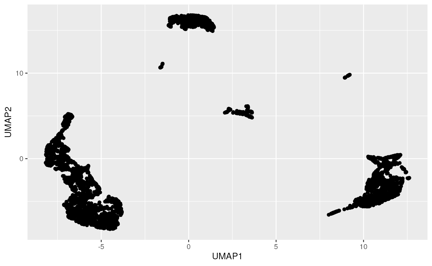
Perform shared nearest-neighbor clustering
(buildSNNGraph()). These nearest neighbors are then used in
community detection algorithms (cluster_walktrap()) to find
similar cells. This represents a faster approach than more traditional
hierarchical clustering.
g <- buildSNNGraph(sce.pbmc, k=10, use.dimred = 'PCA')
clust <- igraph::cluster_walktrap(g)$membership
colLabels(sce.pbmc) <- factor(clust)
Using curated reference data
One approach to cell annotation is to compare expression profiles to
a curated reference data set. We use the reference data derived from
Blueprint and ENCODE data; see browseVignettes("celldex")
for a description of this and other reference datasets.
ref <- celldex::BlueprintEncodeData()
#> see ?celldex and browseVignettes('celldex') for documentation
#> loading from cache
#> see ?celldex and browseVignettes('celldex') for documentation
#> loading from cache
colData(ref) |>
    dplyr::as_tibble()
#> # A tibble: 259 × 3
#>    label.main  label.fine  label.ont
#>    <chr>       <chr>       <chr>
#>  1 Neutrophils Neutrophils CL:0000775
#>  2 Monocytes   Monocytes   CL:0000576
#>  3 Neutrophils Neutrophils CL:0000775
#>  4 HSC         MEP         CL:0000050
#>  5 Neutrophils Neutrophils CL:0000775
#>  6 Monocytes   Monocytes   CL:0000576
#>  7 Neutrophils Neutrophils CL:0000775
#>  8 Monocytes   Monocytes   CL:0000576
#>  9 Neutrophils Neutrophils CL:0000775
#> 10 Neutrophils Neutrophils CL:0000775
#> # ℹ 249 more rows
colData(ref) |>
    dplyr::as_tibble() |>
    dplyr::count(label.main, sort = TRUE)
#> # A tibble: 25 × 2
#>    label.main            n
#>    <chr>             <int>
#>  1 HSC                  38
#>  2 Endothelial cells    26
#>  3 Macrophages          25
#>  4 Neutrophils          23
#>  5 Fibroblasts          20
#>  6 Epithelial cells     18
#>  7 Monocytes            16
#>  8 Smooth muscle        16
#>  9 CD4+ T-cells         14
#> 10 Adipocytes            9
#> # ℹ 15 more rows
Annotate our data using the ‘main’ label for cell type
library(SingleR)
## assign each cell in sce.pbmc to a type
pred <- SingleR(test=sce.pbmc, ref=ref, labels=ref$label.main)
pred |>
    dplyr::as_tibble(rownames = "cell_id")
#> # A tibble: 4,300 × 29
#>    cell_id            scores.Adipocytes scores.Astrocytes scores.B.cells
#>    <chr>                          <dbl>             <dbl>          <dbl>
#>  1 AAACCTGAGAAGGCCT-1             0.252            0.119           0.288
#>  2 AAACCTGAGACAGACC-1             0.280            0.133           0.335
#>  3 AAACCTGAGATAGTCA-1             0.267            0.149           0.298
#>  4 AAACCTGAGGCATGGT-1             0.212            0.154           0.346
#>  5 AAACCTGCAAGGTTCT-1             0.218            0.155           0.368
#>  6 AAACCTGCAGGATTGG-1             0.244            0.139           0.382
#>  7 AAACCTGCAGGCGATA-1             0.324            0.182           0.484
#>  8 AAACCTGCATGAAGTA-1             0.313            0.167           0.461
#>  9 AAACCTGGTAAATGAC-1             0.149            0.0955          0.195
#> 10 AAACCTGGTACATCCA-1             0.210            0.133           0.421
#> # ℹ 4,290 more rows
#> # ℹ 25 more variables: scores.CD4..T.cells <dbl>, scores.CD8..T.cells <dbl>,
#> #   scores.Chondrocytes <dbl>, scores.DC <dbl>, scores.Endothelial.cells <dbl>,
#> #   scores.Eosinophils <dbl>, scores.Epithelial.cells <dbl>,
#> #   scores.Erythrocytes <dbl>, scores.Fibroblasts <dbl>, scores.HSC <dbl>,
#> #   scores.Keratinocytes <dbl>, scores.Macrophages <dbl>,
#> #   scores.Melanocytes <dbl>, scores.Mesangial.cells <dbl>, …
pred |>
    dplyr::as_tibble() |>
    dplyr::count(labels)
#> # A tibble: 9 × 2
#>   labels           n
#>   <chr>        <int>
#> 1 B-cells        578
#> 2 CD4+ T-cells   815
#> 3 CD8+ T-cells  1358
#> 4 DC               1
#> 5 Eosinophils      1
#> 6 Erythrocytes     8
#> 7 HSC             14
#> 8 Monocytes     1258
#> 9 NK cells       267
We can now color our UMAP with predicted cell types.
umap_label <-
    umap |>
    dplyr::mutate(cell_type = pred$labels)
ggplot(umap_label) +
    aes(UMAP1, UMAP2, color = cell_type) +
    geom_point()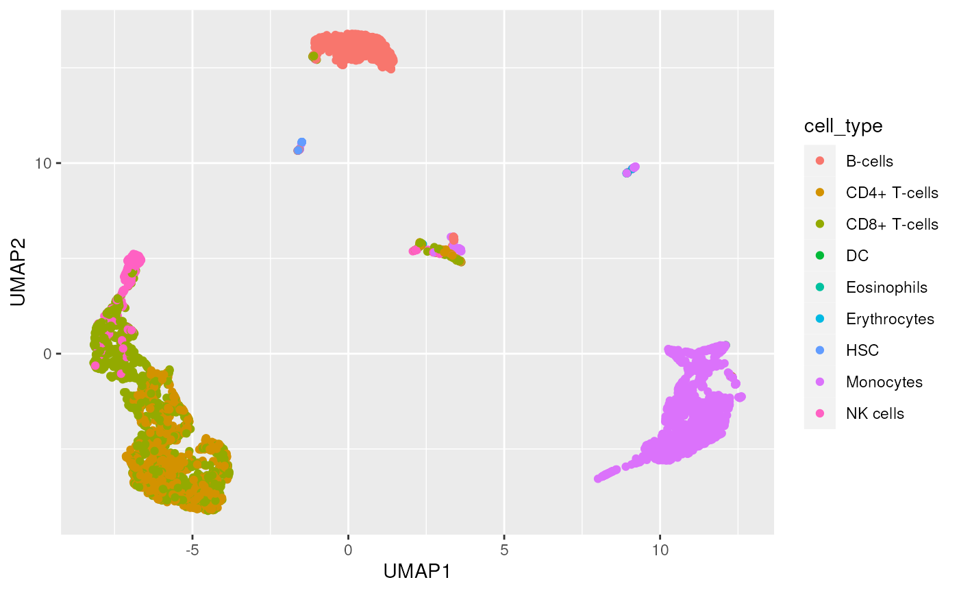
Finaly, visualize the cell annotation. Generally, B-cells and Monocytes are well-annotated, e.g., cells labelled ‘B-cells’ have a strong (yellow) signal only under the B-cell label; CD4+ and CD8+ cells less well-anotated. It is interesting to explore biological reasons that might contribute to this weaker classification.
plotScoreHeatmap(pred)
#> Warning: useNames = NA is deprecated. Instead, specify either useNames = TRUE
#> or useNames = TRUE.

#> Warning: useNames = NA is deprecated. Instead, specify either useNames = TRUE
#> or useNames = TRUE.

#> Warning: useNames = NA is deprecated. Instead, specify either useNames = TRUE
#> or useNames = TRUE.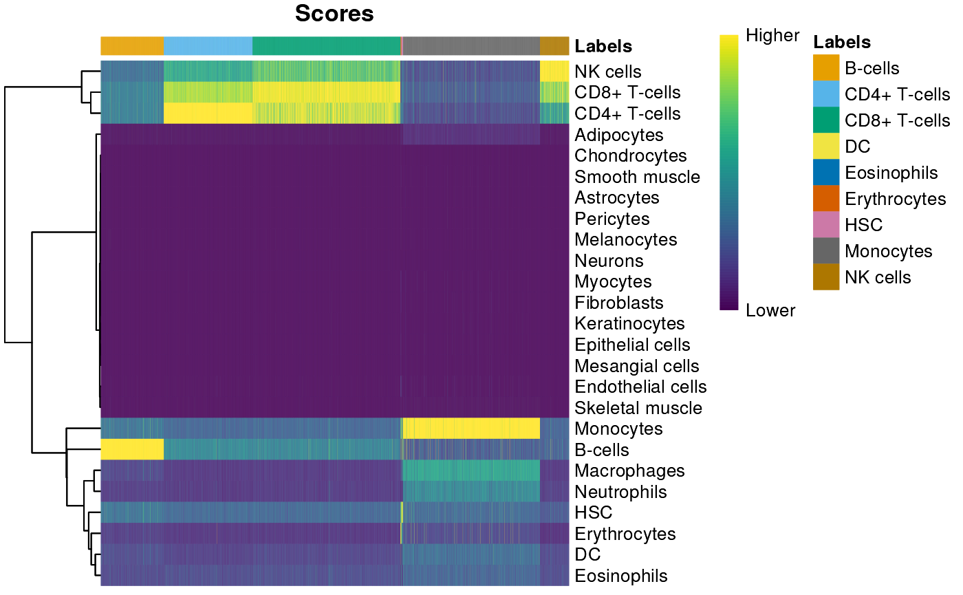
Session information
This document was produced with the following R software:
sessionInfo()
#> R version 4.3.0 (2023-04-21)
#> Platform: x86_64-pc-linux-gnu (64-bit)
#> Running under: Ubuntu 22.04.2 LTS
#>
#> Matrix products: default
#> BLAS:   /usr/lib/x86_64-linux-gnu/openblas-pthread/libblas.so.3
#> LAPACK: /usr/lib/x86_64-linux-gnu/openblas-pthread/libopenblasp-r0.3.20.so;  LAPACK version 3.10.0
#>
#> locale:
#>  [1] LC_CTYPE=en_US.UTF-8       LC_NUMERIC=C
#>  [3] LC_TIME=en_US.UTF-8        LC_COLLATE=en_US.UTF-8
#>  [5] LC_MONETARY=en_US.UTF-8    LC_MESSAGES=en_US.UTF-8
#>  [7] LC_PAPER=en_US.UTF-8       LC_NAME=C
#>  [9] LC_ADDRESS=C               LC_TELEPHONE=C
#> [11] LC_MEASUREMENT=en_US.UTF-8 LC_IDENTIFICATION=C
#>
#> time zone: Etc/UTC
#> tzcode source: system (glibc)
#>
#> attached base packages:
#> [1] stats4    stats     graphics  grDevices utils     datasets  methods
#> [8] base
#>
#> other attached packages:
#>  [1] SingleR_2.3.4               celldex_1.11.1
#>  [3] scran_1.29.0                EnsDb.Hsapiens.v86_2.99.0
#>  [5] ensembldb_2.25.0            AnnotationFilter_1.25.0
#>  [7] GenomicFeatures_1.53.0      AnnotationDbi_1.63.1
#>  [9] scater_1.29.0               ggplot2_3.4.2
#> [11] scuttle_1.11.0              DropletUtils_1.21.0
#> [13] SingleCellExperiment_1.23.0 SummarizedExperiment_1.31.1
#> [15] Biobase_2.61.0              GenomicRanges_1.53.1
#> [17] GenomeInfoDb_1.37.1         IRanges_2.35.1
#> [19] S4Vectors_0.39.1            BiocGenerics_0.47.0
#> [21] MatrixGenerics_1.13.0       matrixStats_1.0.0
#> [23] DropletTestFiles_1.11.0
#>
#> loaded via a namespace (and not attached):
#>   [1] RcppAnnoy_0.0.20              later_1.3.1
#>   [3] BiocIO_1.11.0                 bitops_1.0-7
#>   [5] filelock_1.0.2                tibble_3.2.1
#>   [7] R.oo_1.25.0                   XML_3.99-0.14
#>   [9] lifecycle_1.0.3               edgeR_3.43.4
#>  [11] rprojroot_2.0.3               lattice_0.21-8
#>  [13] magrittr_2.0.3                limma_3.57.4
#>  [15] sass_0.4.6                    rmarkdown_2.22
#>  [17] jquerylib_0.1.4               yaml_2.3.7
#>  [19] metapod_1.9.0                 httpuv_1.6.11
#>  [21] RColorBrewer_1.1-3            DBI_1.1.3
#>  [23] zlibbioc_1.47.0               Rtsne_0.16
#>  [25] purrr_1.0.1                   R.utils_2.12.2
#>  [27] RCurl_1.98-1.12               rappdirs_0.3.3
#>  [29] GenomeInfoDbData_1.2.10       ggrepel_0.9.3
#>  [31] irlba_2.3.5.1                 pheatmap_1.0.12
#>  [33] dqrng_0.3.0                   pkgdown_2.0.7
#>  [35] DelayedMatrixStats_1.23.0     codetools_0.2-19
#>  [37] DelayedArray_0.27.5           xml2_1.3.4
#>  [39] tidyselect_1.2.0              farver_2.1.1
#>  [41] ScaledMatrix_1.9.1            viridis_0.6.3
#>  [43] BiocFileCache_2.9.0           GenomicAlignments_1.37.0
#>  [45] jsonlite_1.8.5                BiocNeighbors_1.19.0
#>  [47] ellipsis_0.3.2                systemfonts_1.0.4
#>  [49] tools_4.3.0                   progress_1.2.2
#>  [51] ragg_1.2.5                    Rcpp_1.0.10
#>  [53] glue_1.6.2                    gridExtra_2.3
#>  [55] SparseArray_1.1.10            xfun_0.39
#>  [57] dplyr_1.1.2                   HDF5Array_1.29.3
#>  [59] withr_2.5.0                   BiocManager_1.30.21
#>  [61] fastmap_1.1.1                 rhdf5filters_1.13.3
#>  [63] bluster_1.11.1                fansi_1.0.4
#>  [65] digest_0.6.31                 rsvd_1.0.5
#>  [67] R6_2.5.1                      mime_0.12
#>  [69] textshaping_0.3.6             colorspace_2.1-0
#>  [71] biomaRt_2.57.1                RSQLite_2.3.1
#>  [73] R.methodsS3_1.8.2             utf8_1.2.3
#>  [75] generics_0.1.3                rtracklayer_1.61.0
#>  [77] prettyunits_1.1.1             httr_1.4.6
#>  [79] S4Arrays_1.1.4                uwot_0.1.14
#>  [81] pkgconfig_2.0.3               gtable_0.3.3
#>  [83] blob_1.2.4                    XVector_0.41.1
#>  [85] htmltools_0.5.5               ProtGenerics_1.33.0
#>  [87] scales_1.2.1                  png_0.1-8
#>  [89] knitr_1.43                    rjson_0.2.21
#>  [91] curl_5.0.1                    cachem_1.0.8
#>  [93] rhdf5_2.45.0                  stringr_1.5.0
#>  [95] BiocVersion_3.18.0            parallel_4.3.0
#>  [97] vipor_0.4.5                   restfulr_0.0.15
#>  [99] desc_1.4.2                    pillar_1.9.0
#> [101] grid_4.3.0                    vctrs_0.6.3
#> [103] promises_1.2.0.1              BiocSingular_1.17.0
#> [105] dbplyr_2.3.2                  beachmat_2.17.8
#> [107] xtable_1.8-4                  cluster_2.1.4
#> [109] beeswarm_0.4.0                evaluate_0.21
#> [111] cli_3.6.1                     locfit_1.5-9.8
#> [113] compiler_4.3.0                Rsamtools_2.17.0
#> [115] rlang_1.1.1                   crayon_1.5.2
#> [117] labeling_0.4.2                fs_1.6.2
#> [119] ggbeeswarm_0.7.2              stringi_1.7.12
#> [121] viridisLite_0.4.2             BiocParallel_1.35.2
#> [123] munsell_0.5.0                 Biostrings_2.69.1
#> [125] lazyeval_0.2.2                Matrix_1.5-4.1
#> [127] ExperimentHub_2.7.1           hms_1.1.3
#> [129] sparseMatrixStats_1.13.0      bit64_4.0.5
#> [131] Rhdf5lib_1.23.0               KEGGREST_1.41.0
#> [133] statmod_1.5.0                 shiny_1.7.4
#> [135] highr_0.10                    interactiveDisplayBase_1.39.0
#> [137] AnnotationHub_3.9.1           igraph_1.5.0
#> [139] memoise_2.0.1                 bslib_0.5.0
#> [141] bit_4.0.5